Overview
The motion planning subsystem utilizes information from a semantic map of the road in concert with an understanding of how that relates to dynamic limits on the vehicle, such as in its speed and acceleration, to plan a path from the vehicle’s current state to its target.
In the spring this was done through a rapidly-exploring random tree (RRT) that shoots potential new states based on feasible control inputs. Variations and modifications to the limits presented in the map were used to decrease planning time, such as projecting speed limits out from the target to require all points can feasibly approach and meet the local limitations set around the target.
At the conclusion of the spring semester, the performance limitations of Shooting RRTs for this application became apparent as the planner had to become overly constrained to avoid oscillations and was expected to be too slow even when ported from MATLAB to C++. For the fall semester then, a weighted A* planner was developed which was inspired by lattice planners presented by Dr. Pivtoriko in his PhD Thesis. Additional description can be found here.
Spring 2020 Development
March 24th, 2020
Ahead of Progress Review #3, we completed the initial implementation and basic testing of the code base for simulation. This included random map generation capabilities along with a simple version of the shooting RRT planner. Certain improvements over the base functionality were also completed such as implementing and testing a progression of distance metrics culminating in one where distance in the direction of motion is cheap and otherwise costly.
March 31st, 2020
Over the week a variety of capabilities were added and refined. One of those is the inclusion of generating the trajectory from the best path. Since each shot is able to record the steps it takes, the trajectory is simply a collation of these states. This one-pass method means no recomputing along the path is necessary. The system now also builds in capability to change the target node between runs meaning that the planner can now be used online. One final major change is the inclusion of limitations based on proximity to the target. What this does is set the speed limit of a location based on its distance from the target in a way that means it is feasible to be within the required speed limit. This reduces the amount of backtracking necessary greatly reducing the planning time and necessary iterations, especially if a significant slowdown was necessary.
April 3rd, 2020
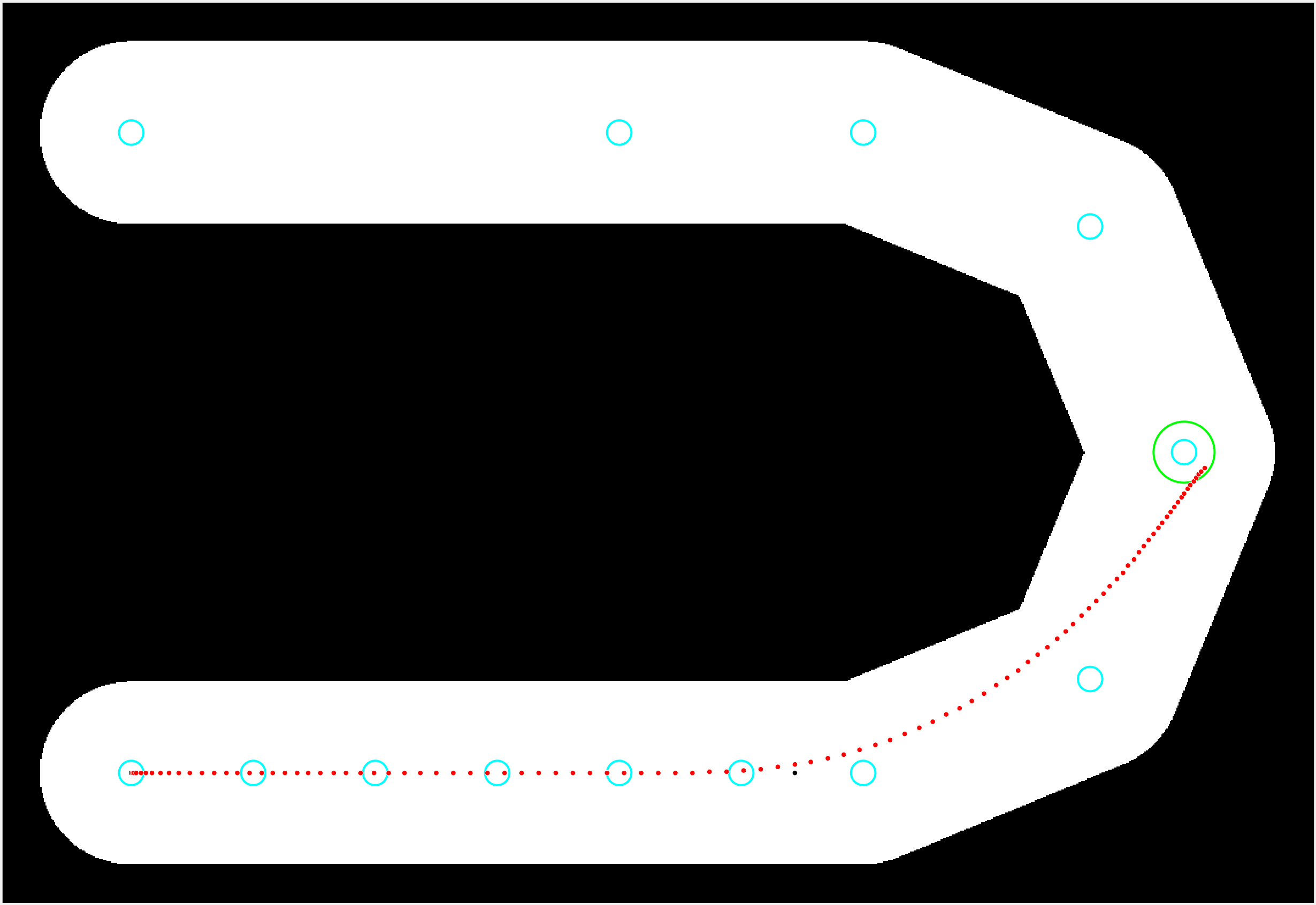
Below is an image representing the status of our planner. This features parameter tuning for more robust and roughly 5x faster (by number of iterations) planning when successful. The vehicle starts in the lower-left cyan circle with heading to the right and zero velocity. The trajectory (red) exhibits how the planner chose to avoid the first two puddles in the lower-left. For the first one it moved out of the way and the second it needed to slow down (more densely placed trajectory points) before going around. For the third puddle, we can see that it decided to slow down and drive through rather than go around. This illustrates one of the key differences between our scenario and normal ones. We are not treating puddles as pure obstacles but rather a different kind of traversable terrain, one that needs to be taken more slowly. Finally, with the target goal being the circles in the upper right we can see the vehicle slow down to be within the velocity threshold. The black dots throughout the road represent nodes in the tree and exemplify the exploratory nature of the algorithm.

April 12th, 2020
The first image below presents some of the developments made to the planning subsystem in the past week. Visually this can be seen in the off-road sections being marked in black as opposed to the blue above, the space around waypoints included in the road are rounded so that no point on the road is more than three-quarters of a meter from the centerline. Behind the scenes, though, significant work was done in terms of improving the planner and tuning many of the different parameters that drive the characteristics of the system. Some of the recent work has included trajectory generation, intermediate waypoint utilization, online planning capacity, smarter sampling, tuning distance metrics, projecting speed limits from the target, breaking out lateral and longitudinal acceleration, rejecting non-improving shots, measuring the distance along the road, and more representative contact limits assessment, among other minor changes. Previously the planner only expanded the tree and selected a final node. Now the shooting system records the steps it takes, which are timed with the desired trajectory frame rate, and the planner collates these together from the selected leaf node to the root. This resulting sequence of frames forms the trajectory. It was possible to provide additional intermediate waypoints before, but they were not used by the planner, except to build the map itself. Now the planner uses the waypoints to better guide the planning around corners so as not to get stuck trying to plan to a target that may be around a bend. Offline planning was really the only way the prior version of the planner could be used. It is now possible to change the target waypoint to be any of the ones given, selected by index, whereas before the last waypoint was assumed to be the target. What this means is that the outer loop that calls the planner can periodically move the target down the road as the vehicle move. In this way, an arbitrarily long and complex sequence of waypoints can be planned through overtime were are tasks such as lapping a loop or crossovers would not have worked as intended and arbitrarily long paths would have been intractable. The sampling itself also helps this as the region where sample points can be taken is restricted to the area around and ahead of the vehicle on the path. Switchback cases provide an obvious example of why sampling from the entire road can be counterproductive. The distance metrics have not changed in style, but have now been refined by a visualization we made to match the intent of the distance metric. A depiction of the level set of our current distance metric can be seen in the second image below. Backtracking in the tree presented an easy way to have the planner slow down for a target or puddle, but it also resulted in exponentially more computation based on the speed difference of the vehicle and the threshold. To speed up this process, we added a projected speed limit out from the target waypoint such that the planner rejects shots that would not result in enough slow down to meet the target’s limits upon arrival. An example of the speed limit can be seen in the third image below. Previous map limits had only specified an absolute acceleration limit. This has been broken out into lateral and longitudinal acceleration for realism and to better constrain the planner to our system requirements. In some scenarios before, where the nearest point to the target couldn’t produce shots that are closer than it a line would form ahead of that node and waste a significant number of iterations. Now the system rejects any shots that don’t improve on the node they are expanding to avoid this waste. For the above-mentioned sampling region, it’s necessary to measure distance along the road and so we added this capability. Other aspects of planning may make use of this in the future as well such as for scaling acceleration ranges. Finally, the planner used to only check the safety of a point at the center of the vehicle, but now that check is made at four points, each representing one of the wheel contact patches. This allows, theoretically, for bridging small puddles in the future, for example, and is generally more realistic.
In addition to the above improvements to the planner, the subsystem was also changed to output its generated trajectory to the associated ROS node as per our ROS architecture. This allows for better emulation of the physical system as it will be implemented on the robot while working in simulation. The ROS architecture diagram can be seen on the Interface page.

April 18th, 2020
Ahead of the SVD demonstrations, various tuning improvements were made and testing completed. In addition to general tuning of all parameters, the planner was used to output test trajectories that the robot could be given to follow as part of physical testing. These test trajectories spanned a variety of characteristics of the trajectories that are necessary for the SVD demonstrations and were designed to allow for testing to build up to the final demonstration. In this way, there were tests that drove various straight-ahead distances with different top speeds as well as others that included a U-turn as a precursor for the SVD 2 demonstration. One additional change was made where a limit was set on the number of times that a single node could be expanded. This helps the planner from getting stuck by removing distracting nodes that may be anchored by unuseful children.
April 25th, 2020
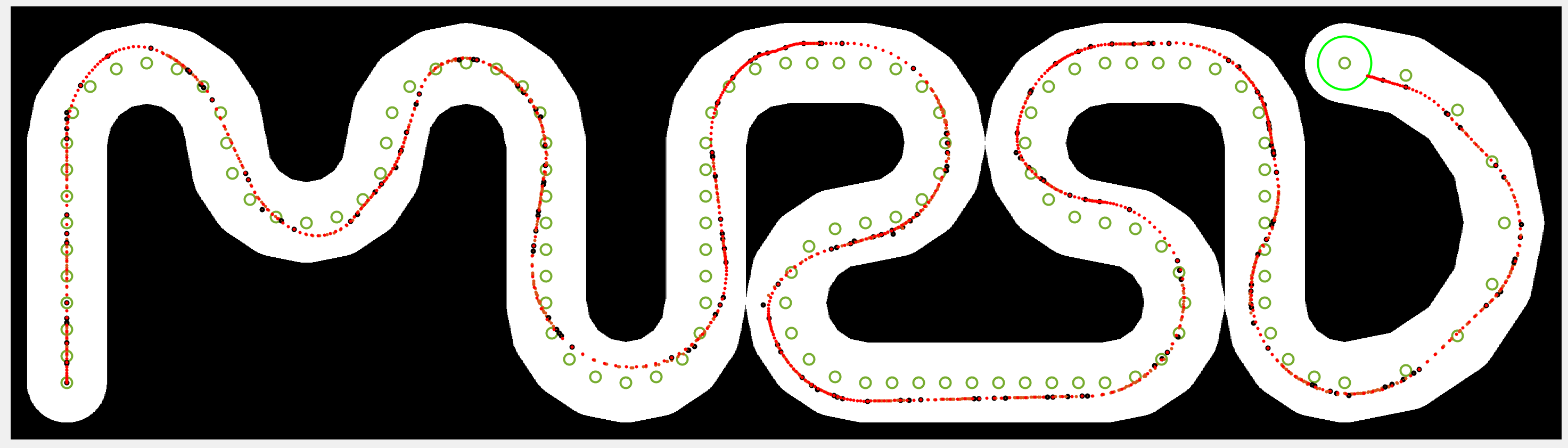
Based on feedback from SVD further improvement was made in the form of a new distance metric where the distance along the road as well as the heading relative to the centerline are incorporated to try and remove lateral oscillations from being incorporated into the trajectory. Additionally, general tuning of the planning parameters was performed with new testing trajectories generated ahead of the field testing session for SVD encore. As a long duration test, a road that spells MRSD was planned on and subsequently followed using the controller in simulation. Below is the resulting image of the planned trajectory.
Fall 2020 Development
September 30th, 2020
By the start of the semester, we had outlined the details of the system we wanted to implement, as laid out here. Developing this work began in September where the base A* planner was repurposed from one of our member’s implementation for 16-782’s Homework 1. This base used hashes as references to planning nodes located in the open and closed set. A custom priority queue based on merge sorting was also implemented to facilitate the selection of the next node to expand.
October 15th, 2020
With this weighted A* base multiple capabilities were added on top to utilize it. One was the pregeneration of motion primitives for use in expanding nodes. See below for an image of a set of motion primitives. These motion primitives are transformed into the state of the expanding node and the resulting states from the motion primitives along with their associated trajectories are added to the priority queue. Footprints for each motion primitive are also generated. These represent every cell in the map that the robot will contact with its wheels and are used to verify that the motion primitive is valid and does not go off the road or exceed velocity limitations. This work was lead by Braden Eichmeier as part of the 16-782 final project. 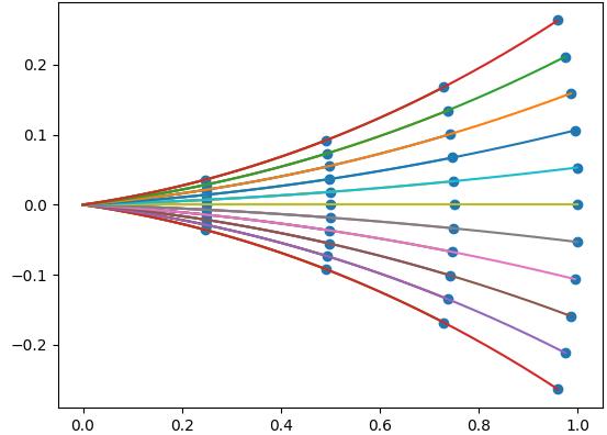
October 20th, 2020
Another necessary capability we were working on in parallel was generating the heuristic map for use by the A* algorithm. This differed from the initially proposed solution in that the implementation generates this map online. The reason for this is so that the heuristic map takes into account the map of puddles provided by the Terrain Comprehension subsystem. More specifically, the heuristic map is generated by taking an intermediate waypoint, selected for being the first beyond the planning horizon, and performing backward Dijkstra from there where the cost for each cell is the time it would take the robot to travel across that cell at the maximum speed allowed for that cell. Without utilizing puddle information, local minima would be created ahead of puddles which would greatly increase the number of nodes expanded and thus time for planning. This work was lead by Shaun Ryer as part of the 16-782 final project.
November 1st, 2020
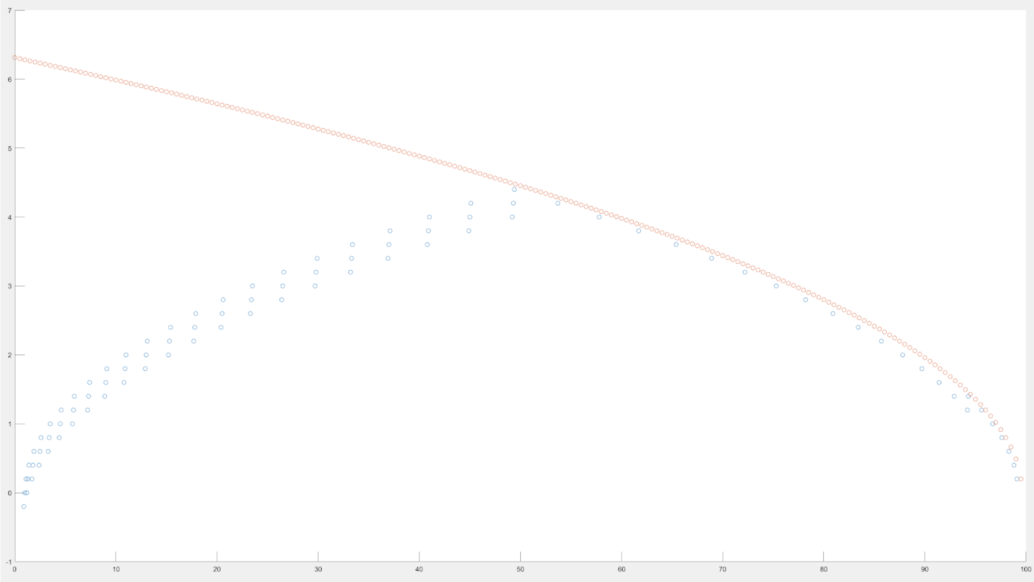
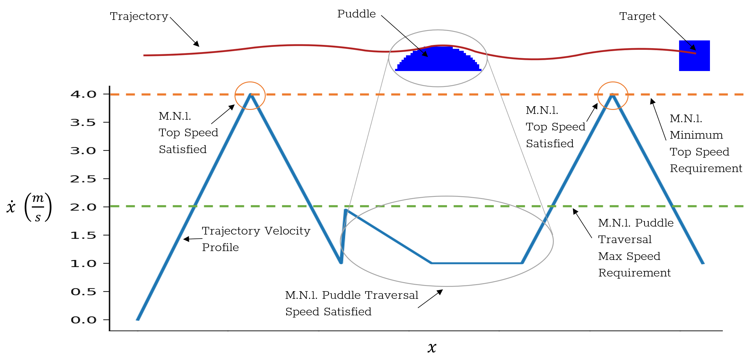
As part of developing the planner, we set up a testing environment for offline planning. Two example maps can be seen below. In order to make sure the planner was abiding by the velocity limitations, we visualized the velocity profiles, as seen in the third image below. With this offline testing environment and verifications, we were able to iterate on the planner until the physical platform was ready. In recognition that the planning code would be moved to the physical robot and moved into a ROS environment, we sought to emulate the interface that would be most convenient with ROS when developing the test environment. Specifically, this meant loading parameters from a yaml file and then porting them into XMLRpcValue type which matches the output from retrieving ROS parameters with roscpp. Additionally, the maps loaded for testing were converted to match the format that would come through the OccupancyGrid message type used by the ROS nodes.

November 15th, 2020
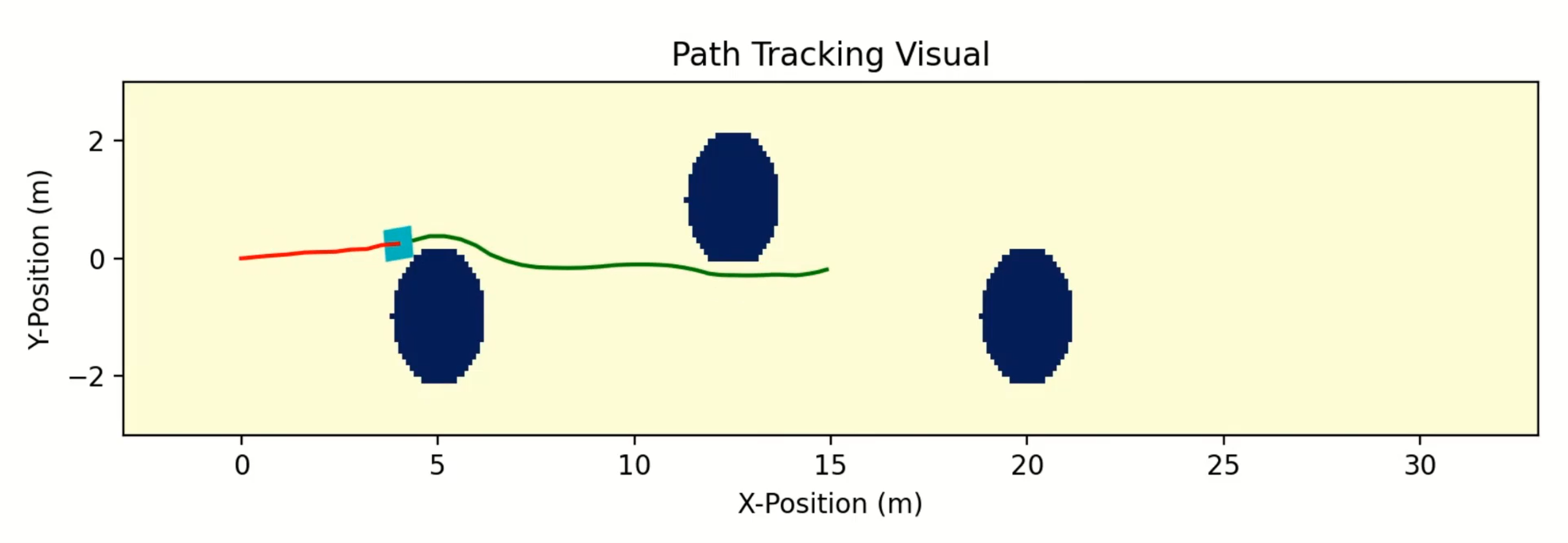
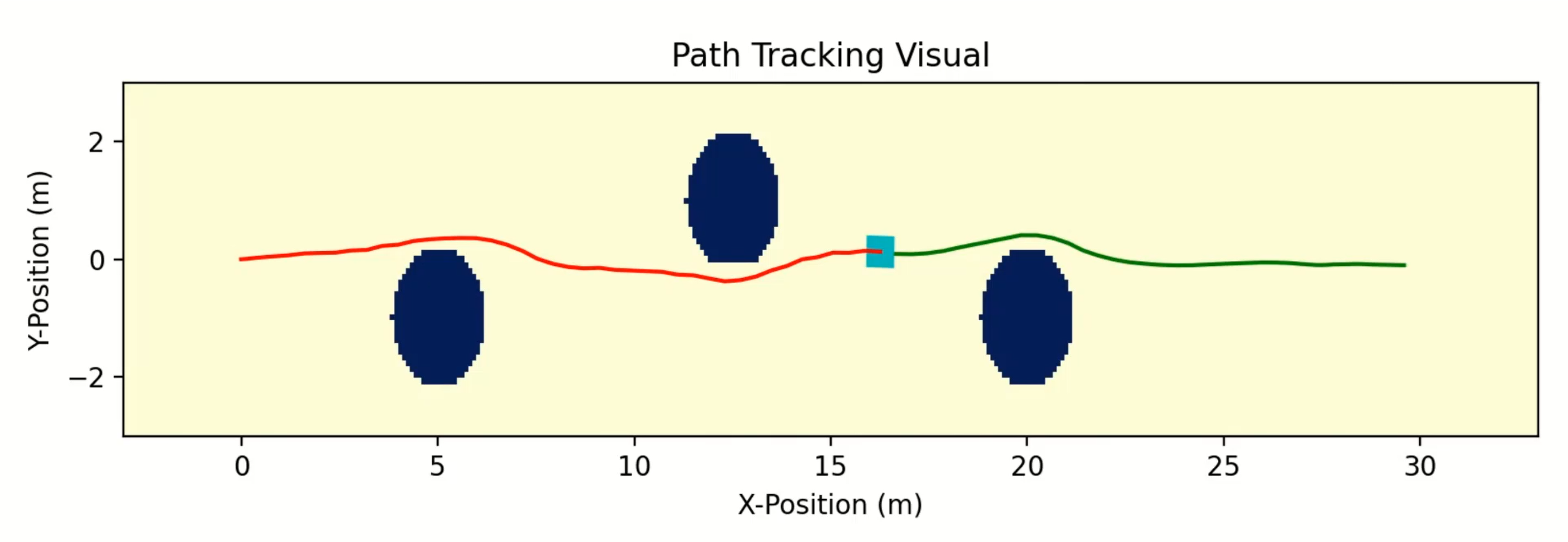
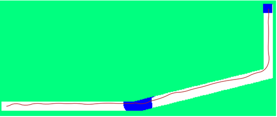
Starting in November we were able to test the planner on the physical robot. Part of making this possible was developing and testing the ROS planning node such that it was able to use the same interface as the testing environment with the map and state values it received from the map synthesis and localization nodes, respectively. Similarly, once the ROS node was set up we set up a visualization node that emulated the localization node and along with the dummy map synthesis node allowed for testing the planner in online mode. A video demonstration of online planning can be seen below. The first image below shows a frame from when the planner’s planning horizon only reaches an intermediate waypoint and while it is navigating around the first puddle. The second image shows the planner reaching all the way to the final waypoint while navigating around the final puddle. In both images and the video, the green line represents the planned trajectory. The red line is the trajectory traveled by the robot. Dark blue regions are puddles. The cyan box represents the vehicle state.