The Terrain Comprehension subsystem perceives adverse terrain and includes the classification, segmentation, and localization pipelines, along with a resulting map output that shows the location of the vehicle relative to the terrain. The focus is on detecting wet road, which includes puddles, versus dry road, where dry road is considered traversable. The suite of sensors used for this task are a FLIR Grasshopper3 Camera, a UM7 IMU, an RTK GPS, and custom-made encoders. Robot state information and an occupancy grid containing probabilities of wet road are passed to the planning subsystem.

Implementation Overview

Perception

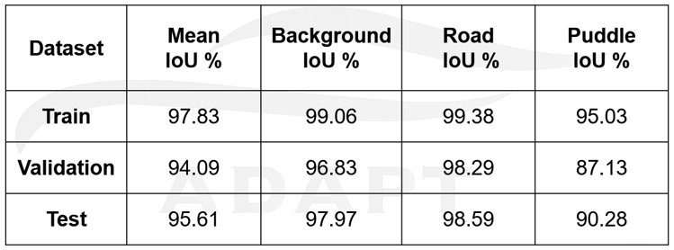
The images from the FLIR camera are sent to a neural network to segment three classes; wet asphalt, dry asphalt, and all other background objects. The network used is called FCHarDNet, and it is a PyTorch implementation of HardNet. The network can segment at 18 FPS after various optimizations were introduced which included downscaling the incoming image and multi-threading the loading and segmenting portions of the code. Below is a table of the Intersection-over-Union (IoU) scores on the training, validation, and test data.

A total of 516 images were collected and manually annotated by the team. These were images taken at the top level of the east campus parking garage of Carnegie Mellon University, as this was to be the location for the Fall Validation Demonstration.

The segmented masks are used for generating the map, which is an occupancy grid of wet road probabilities. The mask is warped based on the the angle at which the camera sits on the car. A checkboard calibration provides the camera intrinsics, which are used in conjunction with the camera angle to create a homography to warp the mask. The warped mask is downscaled to match the resolution of the map, and the oriented and placed on the proper map location using the state values. Subsequent masks are merged by weighting the running average of already calculated wet road locations against the most recent mask received to calculate the final probability value that is stored in the cell.

Localization

The duty of the localization system is to provide accurate and live information to the robot about its current state. The components of the state representation are x, y, θ , ẋ, ẏ, and θ̇ . It also includes acceleration information for each of x, y, and θ , but they are not used by any other sub-
system. The state reference frame is defined as the pose of the robot when localization is started or reset. The frame is offset by a provided initial state, which most of the time is set as zeros. Additionally, the x-axis is set to always be parallel to the long side of the parking garage. In order
to achieve live and accurate information, an Extended Kalman Filter (EKF) is utilized with three different contributing sensors: RTK GPS, IMU, and encoders. This suite of sensors was chosen so that direct measurements of each of the state values used by other systems could be obtained. The
RTK GPS provides location (x and y) information. The IMU provides yaw (θ ) and yaw-rate ( θ̇ ) data. Finally, the encoders provide velocity information, which in conjunction with the yaw of the vehicle, is transformed into the two component velocities ( ẋ and ẏ).

Changes from Spring Semester

The initial perception subsystem design was going to include multiple sensors, including a ZED Stereo Camera, a FLIR Grasshopper3 Color Camera,  a FLIR BOSON 320 Thermal Camera, and Velodyne VLP-16 Puck. The Velodyne Puck (lidar) was ruled out early in the spring semester after an experiment showed that it was nearly impossible to detect wet areas or puddles with the lidar. The point cloud was too sparse to see major differences between wet and dry areas. The thermal camera was also eliminated after viewing the thermal footage. The wet areas were often the same temperature as the dry road since the water had been sitting on the road for a while and the temperatures reached equilibrium state.

The ZED Stereo Camera was fully explored in during the fall semester for use as a classical method to detect puddles. It involved placing polarized filters at different orientations over the two lenses of the stereo camera and calculating features from the resulting image. A Gaussian mixture model was trained to perform segmentation. While the puddle segmentation was relatively accurate, the algorithm was unable to function in real-time. Therefore the ZED Stereo Camera was left out of the perception pipeline, and the only method of vision the system uses is the FLIR monocular camera.

In the spring semester, the neural network used was YOLACT. It was an instance segmentation network, which led to some inaccuracies in segmenting wet road. Additionally, YOLACT was implemented only on a laptop. In the fall semester, a semantic segmentation network FCHarDNet was implemented on the Xavier itself. The training images in the spring semester were gathered from Highland Park and labeled with the free labeling software LabelMe. In the fall, the training images were gathered from the east campus parking garage and labeled with different software provided by a startup company.

Terrain Comprehension Subsystem Progress

January 17th, 2020

Today we tested the Velodyne LiDAR and its ability to detect puddles. We set up an area in the basement of NSH to perform the test. Since there was a drain on the floor just outside of the lab, we filled a bucket of water and poured it near the drain to create a puddle and a large wet area. We placed the lidar on a table in both standard orientation and rotated vertically and inspected the results. There appeared to be a few points in the point cloud that were missing in the puddle area, but it was difficult to notice the absence of those points. It is likely that the output laser reflected away from the puddle and did not come back to the receiver, thus producing a blank spot in the puddle area. We will discuss the options we have with the lidar and how we can use the data to puddles and wet areas.

January 21st, 2020

We have decided not to move forward with the LiDAR, at least for this semester. We will focus on using the ZED stereo camera and using polarized filters to detect puddles and wet areas. The stereo camera will also provide us localization information. We will also be using a neural network to perform segmentation of the images to determine puddle regions.

February 11th, 2020

We have been researching and doing initial implementation of a few neural networks for segmentation, including ShuffleSeg, SegNet, and FasterSeg. We are moving forward with trying ShuffleSet and FasterSeg, as both are more recent works and thus perform segmentation quicker than SegNet, which is a relatively older network.

February 25th, 2020

We again set up an area in the basement of NSH to test the polarization filters with the ZED Stereo Camera.  We placed a horizontally polarized filter on the left lens and a vertically polarized filter on the right lens and captured images of the puddle and wet area. One of the test images we took is shown below. Upon close inspection, the puddle appears darker in the right image compared to the left image. This behavior is what we want, as we would like to use the difference in intensity of the puddles in the two images to detect the puddle.

March 6th, 2020

Today we placed the ZED camera on a mock setup of the enclosure and test drove the car with the polarization filters and collected video. The sun had come out just after a rainstorm, which made it perfect for capturing video. We recorded video in the area just in front of NSH. Again, we were able to see that the left image has lesser intensity compared to the right image. Shown below is the video we recorded.

 

March 17th, 2020

We obtained the FLIR BOSON 320 Thermal Camera from Team Phoenix and started installing the relevant packages on Ubuntu to utilize the camera. We will familiarize ourselves with the packages and later take test video to determine what methods we should use to detect puddles.

March 22th, 2020

We successfully created the disparity map from the ZED stereo images using the test video we took on March 6th. The map essentially depicts how much an object appears to move when viewed from the right lens as compared to the left lens. The disparity map is generated using OpenCV’s function for computing stereo correspondences using a block matching algorithm. This function was used instead of the function in the ZED API because OpenCV’s function has more settings that can be tuned. The next step is to use the disparity to obtain the actual depth associated with each pixel. Show below is a video of the disparity map generated on video taken around NSH.

 

March 28th, 2020

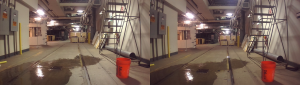
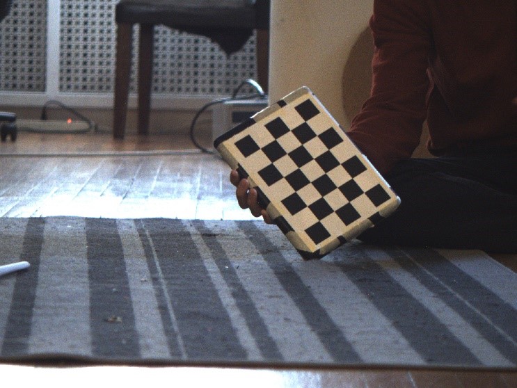
Today we collected test video using the FLIR BOSON 320 Thermal camera. The video was taken when there was sunlight just after a rainstorm, which meant there were a lot of puddles on the road. Since the vehicle enclosure has not been completely assembled, the test video was taken by holding the camera in hand. Since the purpose of this test was to assess the feasibility of using IR data in detecting puddles, the handheld video is sufficient at this time. Shown below is a snapshot from the video of the camera. The puddles show the reflection of the buildings in the background, however they are otherwise the same temperature as the road, which makes them difficult to distinguish without the reflections. Also shown below is a color image for reference to compare with the scene in the IR camera. The next step is to tune the gains on the camera to see if they make the puddles more distinctive, and if they do not, we will likely forego using the IR camera entirely. Shown below is a still frame from the IR camera and the corresponding RGB scene (from a slightly different angle), as well as some of the gathered video.

 

April 5th, 2020

The critical aspects of the vehicle hardware, such as the sensor mounts, were recently completed, so the ZED stereo camera was able to be mounted in its proper position on the car. We went to Highland Park to gather video of puddles for labeling. The sky was overcast and drizzling, so most of the ground was already wet. However, we had to bring our own containers of water to pour on the ground to create puddles. After we returned from Highland Park, each frame of the video was converted into an image, and we began the image labeling process. We used an image labeling software called LabelMe to draw polygons around the two classes of road and puddle.

April 15th, 2020

The labeling process took a few days and we ended up with 200 images. After shuffling the images, 60% of the images were used as the training data set, 20% was used as the validation data set, and the last 20% was used as the test data set. We also settled on implementing a real-time instance segmentation neural network model called You-Only-Look-At-CoefficienTs (YOLACT). This network requires its image labeling format to be the same format as in the COCO dataset, so we first converted our LabelMe annotations to COCO format before training.

We used batch sizes of 2, 4, 8, 16, and 22 and used Resnet50 as the pre-trained weights.  Training took a few days as well, with each member of the group performing some of the training. The Intersection-over-Union (IoU) metric was used to evaluate how well the network segmented puddle and road. We looked at both the average IoU across all frames as well as the percentage of frames that had an IoU above a certain threshold. Shown in the video below is the segmentation of one of the videos collected from Highland Park.

 

April 20th, 2020

We went to Highland Park again to gather more data, and this time, it was a sunny day. The puddles were more distinct this time as compared to last time when it was drizzling. More data was labeled, and our new total of annotated images, which includes the images from the previous trip to Highland Park rose to 310.

April 25th, 2020

Training of YOLACT was performed again, but this time three different pre-trained weights were used for training: Resnet50, Resnet101, and Darknet53. The batch sizes used for training were 2 and 10. Various combinations of these weights and batch sizes were used for training, and the combination with the best Intersection-over-Union (IoU) performance on validation data was selected to use for final evaluation. Darknet53 with a batch size of 2 provided the best results. Shown below is the segmentation of the same video from above, but with improved results.

Since we had already been unable to implement a neural network directly on the Xavier in the spring, over the summer we decided to try to set up a Docker container on the Xavier. The idea is that we would install the appropriate python packages (PyTorch, Torchvision, OpenCV, etc.) in the container and run the neural network in the container.

September 16th, 2020

After doing further investigation into getting YOLACT to evaluate a video within the Docker container, we were unable to come up with a solution. It seems as if OpenCV has trouble running to its full capabilities within the container with respect to video processing.

Since it is critical to get OpenCV working, we decided to try one final time to get YOLACT working directly on the Xavier (not using the Docker Container). Since OpenCV is already installed onto the Xavier’s system Python 3.6 when it is flashed with Jetpack (version 4.4, L4T R32.4.3), we tried to use Python 3.6 for the rest of the necessary packages.

After much digging through forums, we downloaded the following wheel files for PyTorch and Torchvision:

• https://nvidia.box.com/shared/static/c3d7vm4gcs9m728j6o5vjay2jdedqb55.whl 15
• https://nvidia.box.com/shared/static/c3d7vm4gcs9m728j6o5vjay2jdedqb55.whl

These successfully installed and we were able to successfully run YOLACT on the system Python, outside of the docker container. Unfortunately, YOLACT runs at only 5 FPS, so we need to figure out some optimizations to increase the frame rate.

September 26th, 2020

After doing more research, we concluded that it is likely the Xavier just is not computationally powerful enough to run a network like YOLACT at a higher FPS. The benchmarks from the YOLACT paper (and other neural network papers) all use NVIDIA GPUs that are more powerful than the GPU that is on the Xavier. Thus, we decided to search for another network and found one called FCHarDNet (https://github.com/PingoLH/FCHarDNet), which is a PyTorch implementation of HardNet. We were successfully able to implement it on the Xavier.

This initial implementation of FCHarDNet on the Xavier yielded only a 10 FPS segmentation speed, which was too slow for our purposes. We timed each individual section of code that went into the overall segmentation to determine which steps took the longest and if we could improve upon them. The different sections were: image loading, image pre-processing, segmentation, post-processing, and stream display. The segmentation and image loading were the most time consuming portions, thus multi-threading was used to simultaneously segment a frame and load the next frame to be segmented. Additionally, the images were downsampled to a fourth of the original resolution from the FLIR camera. After implementing these optimizations, we achieved an 18 FPS segmentation speed, which is acceptable based on the desired robot speeds and planning horizon. The video below demonstrates the segmentation results. Blue areas are pixels classified as puddle and green areas are classified as road. A third class of “other” is detected by the network as any non-puddle and non-road pixel and is displayed as black.

 

October 15th, 2020

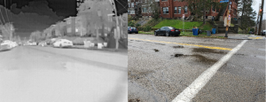
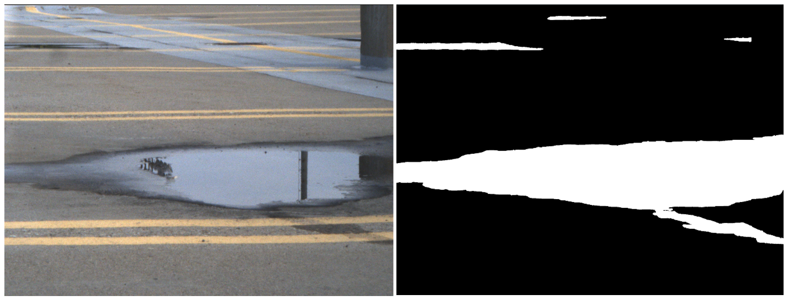
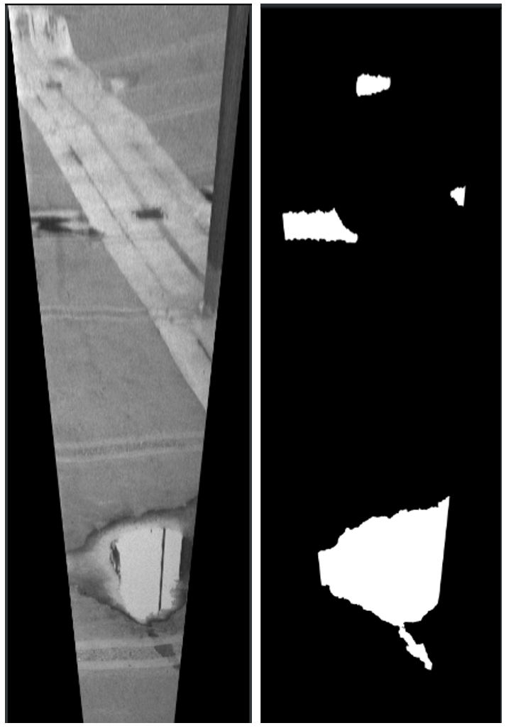
The next part of the perception subsystem after segmentation is map generation. The masks output by the segmentation network are used to generate an occupancy grip map, where the values in the cells of the map are the probabilities of puddles being at those locations. Shown below is an image and the output mask of the segmentation network.

We completed some of the backend code for map synthesis. The first step was to take a perspective transform of the mask by warping it to become a bird’s eye view perspective. This is done through a homography, where the homography is determined by:

H = KRK^-1

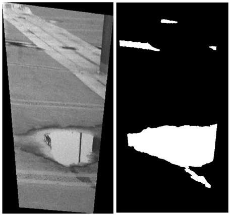
with K being the intrinsics of the camera and R being the rotation matrix corresponding to the rotation about its enter. OpenCV’s perspective transform function then takes this homography and uses it to warp the entire mask. Shown below is the result of warping the mask (the warped image is shown as reference and is not used for actual perception).

Since the intrinsics of the FLIR Grasshopper3 were not readily available, we performed camera calibration using a checkerboard. We took about twenty pictures of the checkerboard at various orientations and places in the image frame. MATLAB’s image process toolbox has a camera calibration tool which takes in the checkerboard images and checkerboard square size as parameters and outputs the intrinsics.

October 20th, 2020

Work was continued on the map generation. We intend on using the IMU to incorporate roll, pitch, and yaw information to use in properly transforming the mask and merging the mask onto the map. The roll and pitch information are used in the transformations, as the changes in camera angle will affect how the warp should look. Thus, the homography is now calculated with this information through:

H=KR_xK^-1R_z

Where R_x is the rotation about the x-axis of the image, and R_z is the rotation about the z-axis of the image. The x, y, and z image axes are pointing right, down, and into the image plane, respectively. Thus, the pitch of the car is a rotation about the x-axis, and the roll angle of the car is a rotation about the z-axis. Shown below is an example warp with roll incorporated. The original image did not have any roll that needed correction, but the result demonstrates the desired effect.

After this warp, the mask is downscaled to match the cell resolution of the map, since the warp has no explicit depth information. For example, if a cell in the map is supposed to represent 0.1m, then the mask is downscaled to match this. The position and yaw information from the state is then used to orient and overlay the warped mask correctly onto the map.

October 29th, 2020

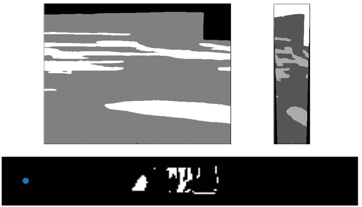
The merging process of the map has been completed. Shown below is the mask, warped mask, and the merging onto an new map. The blue dot represents the robot’s current position. The map is oriented with its x and y axes pointing right and upwards, respectively. So the mask after downscaling must be oriented so that it aligns with how the car is facing in the frame of the map. The yaw information from the IMU is used for this. In the simple case, if the IMU reads a 0° yaw value, then the car is facing the x-axis in the world frame. Therefore, the mask would need to be rotated by 90° clockwise before being merged. The probabilities are calculated with a simple running average of where puddles have been seen up to the current time.

November 15th, 2020

The map generation has been refined after experiencing issues related to speed and accuracy. We decided to slightly change the process for generating map depending on whether we wanted online or offline map generation. For online map generation, we cropped off the a number of rows for the mask to make warping faster. For offline map generation, we leave the mask as normal sized since time does not matter.

We also decided to add in a weighting factor that took into account because we wanted to have more recent masks show affect what appears on the map quickly. This means we have some weighting factor on the existing probabilities and the complimentary weighting factor on the incoming mask.