Based on the functional and cyberphysical architecture, we divide the system into two high-level subsystems — the UAV subsystem and the UGV subsystem.
UAV subsystem
The UAV subsystem can be further divided into three software modules and one hardware module: the navigation module, the tracking and landing module, the global path planning module, and the hardware module. The navigation module ensures the UAV can reach way points specified by GPS coordinates while avoiding simple obstacles. The landing module allows the UAV to be able to land on the UGV’s landing platform. The global path planning module is responsible for calculating the relay point for the UAV and the UGV and an optimal path that the UAV can follow. Lastly, the hardware module consists of the UAV platform itself and the onboard computer.

Figure 1: DJI M100 UAV
Navigation Module
The navigation module allows the UAV to follow GPS way points while avoiding simple obstacles. We used a ROS package called “navigation” for the backbone of this module; it takes in information from odometry and sensor streams and outputs velocity commands to send to the UAV.

Figure 2: ROS Navigation Stack
The navigation stack assumes that the robot is configured in a particular manner in order to run. The diagram above shows an overview of this configuration. The white components are required components that are already implemented, the gray components are optional components that are already implemented, and the blue components must be created for each robot platform. I will go through each of these components, the steps we took to set them up, and how we fine-tune toward our particular robot.
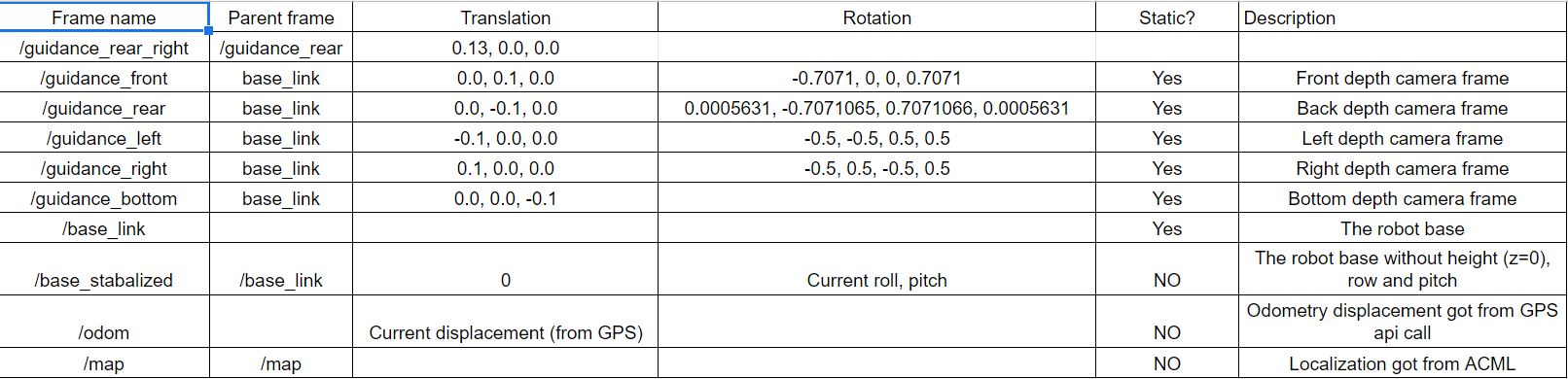
Figure 3: UAV frame transformation relationships
The first component is the transformation configuration. The navigation stack requires the robot to be publishing information about the relationships between coordinate frames such as base frame, sensor frame, and odmetry frame using ROS tf package. The excel screenshot above shows the relationships we defined for each frame. Frames start with “guidance” represents the sensor frames of the five stereo cameras equipped on the UAV. The “base link” frame is the main frame representing the orientation of the UAV. The “base stabilized” frame represents the orientation of the UAV without roll and pitch angles. The “odom” and “map” frame are world-fixed frames based on odometry information and mapping information, respectively.
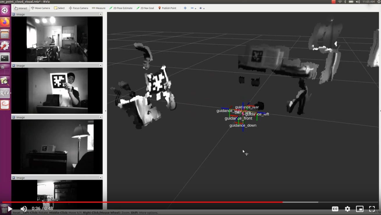
Figure 4: Pointcloud visualization in Rviz
The second component is the sensor information. The navigation stack uses information from sensors to avoid obstacles in the world. In our case, we are using the five stereo depth cameras mounted on the drone. Since the navigation stack assumes these sensors are publishing “LaserScan” messages over ROS. There are three major steps we took to convert raw greyscale stereo images into “LaserScan” messages and feed in the navigation stack. The first step is to extract the intrinsic parameters for each camera. We used a ROS package called “camera calibration” to accomplish this step. The second step is to generate point clouds from stereo image pairs, which we used ROS package “stereo image proc”. We also tuned parameters used by the block matching algorithms which transform the stereo images to pointcloud . The third step is to convert generated pointcloud messages to laserscan messages and publish them. This was accomplished using “pointcloud to laserscan” package and a publisher. The result laserscan and pointcloud are shown as white lines below.
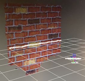
Figure 5: Point cloud and laser scan visualized in Rviz
The third component is odometry information. The navigation stack requires that odometry information be published using ROS tf package. Specifically, the information consists of the UAV’s positions in xy plane, yaw angle, linear velocities in xy plane, and yaw angular velocity. All information can be extracted from callbacks from the GPS and the IMU sensor.
The fourth component is base controller. The navigation stack assumes that it can send velocity commands in base coordinate frame on a specific topic. I implemented a node subscribing to that topic and capable of converting them to motor commands sent to the UAV move base via appropriate API calls.
We are not providing a static map to the path planner and we are not creating one using SLAM on the way either since obstacle avoidance is really not the main focus for this project. In addition, parameters for the costmap and local planner are tuned based on the performance metrics of the UAV.
Lastly, to make navigation as autonomous as possible. We also wrote a high-level Python script in charge of publishing GPS waypoints to the navigation stack and updating the goal if the UAV reached the current way point or the time limit is reached.
The final implementation was tested in a simulation environment using Gazebo (Figure 6), and the UAV is able to reach each of the waypoints or skipped the ones that are invalid (on or too close to the obstacle).
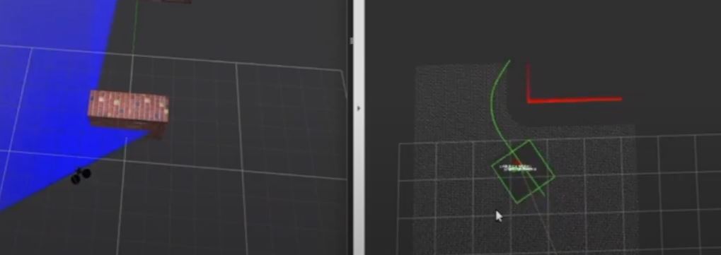
Figure 6: Planned path, costmap and obstacles visualized in Rviz and in Gazebo
Tracking and Landing Module
The tracking and landing subsystem is responsible for tracking and landing on the landing platform marked by Apriltags. It consists of two components: the tracking component and the landing component.
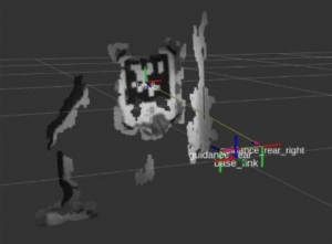
Figure 7: Apriltag Tracking in Rviz
The tracking component is able to recognize the tag from the greyscale or RGB video stream and publish a pose transformation relative to the camera frame. This was done using the ROS package “apriltag ros”. Given a video stream input, the tracking component is able to publish a transformation between the tag frame and the camera frame in real-time. In order to further improve the pose estimation accuracy, we also tested out the detection algorithm with tag bundle which consists of 5 Apriltags instead of one. Using tag bundles increases the pose estimation accuracy since the algorithm will take the average of its location estimations of all tags to minimize the error. The algorithm is able to identify each of the tag from the greyscale video stream but they are identified as one in coordinate frame transformation.
The landing component is responsible to generate velocity commands to the UAV motor controller based on the pose estimation published by the tracking component. This was done using a PID controller with position error in x, y, and yaw as input and control efforts in pitch, row, and yaw as output. The gains of the controller were tuned using a combination of the Ziegler–Nichols method and trail and error. In this case, it’s a balance between how fast the UAV can converge to the center of the tag and the steady-state error. Our current set of gains tilts toward stability over speed. The control efforts are directly published to the UAV motor through API calls.

Figure 8: Rviz visualization of Landing process in Gazebo and PID control graphs
Global Path Planning Module
The global path planner allows the UAV to generate waypoints and path that takes the current batter statuses and locations of both the UAV and the UGV into account. The goal of the global path planner is to find a path that for the UAV to get to the UGV in as little time as possible so neither the UAV nor the UGV runs out of battery. In addition, the rally point should be an open area that is safe for landing. As a result, the UAV should stay connection for any updates from the UGV about the landing point clearance status and be ready to reschedule if anything changes.
According to our plan, we are not going to start implementing the global path planner until the fall semester, so we currently don’t have any progress updates on this specific module.
Hardware Module
The UAV hardware module consists of two components: the UAV platform itself and the onboard computer. For the UAV, we chose the DJI M100, because it’s highly customizable and its software APIs are well-documented. It comes with a GPS sensor, an IMU, five stereo depth cameras and five ultra-sonic sensors. We assembled it together once we received it early in the semester, and we also performed a outdoor field test just to make sure everything was working properly. We are not planning to do any additional modifications other than the landing gear extension which pairs with the UGV landing platform (Please see the landing platform module under the UGV subsystem section for more details about the landing gear extension).
For the onboard computer we chose the Nvidia Jetson TX2. In order to fit it onto the UAV, we replaced its original extension board with a much smaller third-party extension board. We also paired it with a step-down voltage, since the output voltage from the battery was too high. Lastly, there’s this enclosure for the computer, just to protect it from any sorts of collision damages. Below are all the components for the onboard computer and its final form after putting everything together: TX2 (top-left), voltage converter (top-right), extension board (middle-left), and enclosure (middle-right).
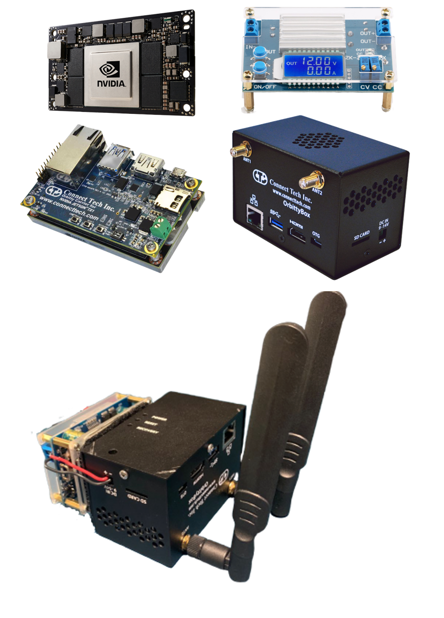
Figure 9 Onboard computer components and its final form
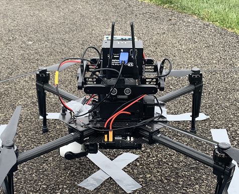
Figure 10 UAV with the onboard Computer
UGV subsystem
The UGV subsystem includes three important modules: Mapping, navigation and decision making to choose landing point modules. The mapping module will create a 2-D occupancy grid map from Velodyne and pose data collected by mobile robot (SLAM). Then the UGV could run autonomous navigation avoiding obstacles by means of global and local path planning towards the landing point based on decision making.

Figure 11 UGV subsystem overview
Mapping
The mapping module uses OpenSlam’s Gmapping to provide laser-based SLAM (Simultaneous Localization and Mapping), as a ROS node called slam\_gmapping.
We can launch RViz and add a display type called Map and the topic name as /map. After that, we can start moving the robot inside the world by using key board teleoperation, and we can see a map building according to the environment.
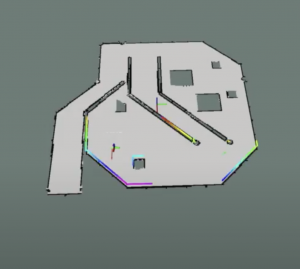
Figure 12 Completed Map in Rviz
Navigation
Based on the static map created from the laser scan data, the robot can autonomously navigate from any pose of the map using amcl and the move\_base nodes. The first step is to create a launch file for starting the amcl node.
Similar to the navigation stack of the UAV, the navigation stack package will feed the sensor transformation and odometry data to the planner. Then it publishes map and sensor data to avoid obstacles as source. By calculating the global and local trajectory with cost map, the stack sends velocity commands to the robot.
As shown in Figure below, the navigation stack generate the global path for the UGV. During this stage, the UGV will follow several waypoints, of which the errors are within 0.3 meters. Also, within the test map, the UGV will reach a landing point candidate within 60s.

Figure 13 Global Path for navigation
Decision Making to choose a landing point
Based on the map generated in SLAM, an optimal landing point algorithm is designed for the UAV landing on the UGV.
The key idea behind the algorithm was that we check whether there is a large enough circle existing, which was centered at a position randomly sampled from the given map. The radius circle had to reach the threshold for safe landing. The sampling part was triggered by RRT, or RRT-connect algorithm, in order to speed the process up. After that, since the map was an occupancy grid, we had to discretize the circle to check whether each point inside the circle is valid. In order words, the cell is free of obstacles. If we found a valid sample point, we would use this point for the UGV to navigate, which helped update the map for the next step.

Figure 14 Second Landing Point Navigation
Using this algorithm, the UGV marks the first landing point candidate as unreasonable, which is the end of the green line. The reason is that there are several blocks around the landing point, which is not suitable for landing. Then the UGV will go to the second point, which is the end of the green line in Figure
Landing Module
The landing module is implemented as a hardware redundancy to reduce the UAV landing error to a millimeter level. The landing module is separated into two sub-modules, with each sub-module installed onto the UAV and the UGV respectively. A connector and a permanent magnet are connected to the UAV, and a receptor with an electromagnet enclosed will be connected to the UGV.

Figure 16: Landing Module Explode View
During the landing process, as the UAV approaches the receptor by tracking the apriltag, the electromagnet will be switched on and exerting an absorption force to the permanent magnet installed on the UAV. The cone-shape receptor will guide the UAV connector slide into the place. With the assistance of this landing module, we can reduce the landing error from the tens-of-centimeter level to the millimeter level, which makes wireless charging possible for the UAV.
To model, analyze, and test the performance of the mechanical design of the landing module, we measured the dimension and performance of each component. The two most important factors directly affecting the landing performance are the inner diameter (ID) of the receptor, and the effective absorbing range of the electromagnet: we assume that within the effective absorbing range, the larger the receptor ID, the easier the landing performance is, and the higher landing success rate the system can achieve. Within a distance of 12cm, the activated electromagnet can effectively attract the permanent magnet, and the receptor ID is currently set to be 10cm. In this setting, 80% landing success rate can be achieved. Additionally, there is a huge space buffer above the receptor upper surface to the effective absorbing range. To further improve the landing performance, we plan to lift the receptor wall up and increase the receptor ID from 10cm to 16cm.

Figure 16: Cross Section of Landing Module