February 11, 2020 – Initial test flight
We finished assembling the drone, which is a DJI M100. It comes with sensors including a GPS, a compass, an IMU, five sets of stereo cameras and a Gimbal camera. To make sure everything works properly, we also performed an outdoor test flight for basic maneuverability including taking-off, hovering, movement in all six axes and landing.
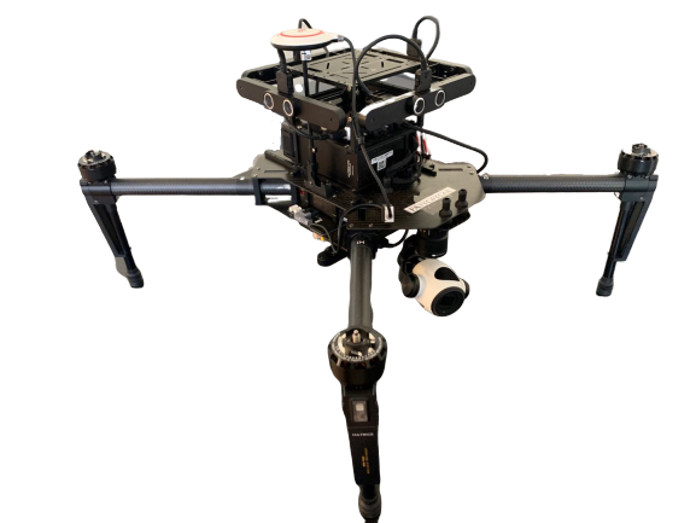
Figure 1. UAV subsystem, DJI M100
February 17, 2020 – Initial GPS mission under simulation
Today we were able to set up and run a simple simulation on a GPS waypoint-following mission using the SDK and the DJI simulator.
Unlike our simulation for the UGV subsystem, the DJI simulator requires the drone to be connected with the PC while the simulation is running. Specifically, the drone was connected with a Linux laptop, serving as the ROS onboard computer, and a PC, where we run the simulator. DJI has a very powerful SDK available to the developer. Tasks like taking-off, waypoint following and returning home are well-supported and documented. In the simulation we performed, the UAV was able to take-off to a given altitude, run by several waypoints specified by GPS coordinates, returning home at a lower altitude and land at where it took off. We conclude that the current automatic flight-control API is sufficient for our project except for the landing part where a much higher accuracy is required. However, eventually, we would have to transfer our simulation environment into Gazebo, as that’s where the UGV simulates.
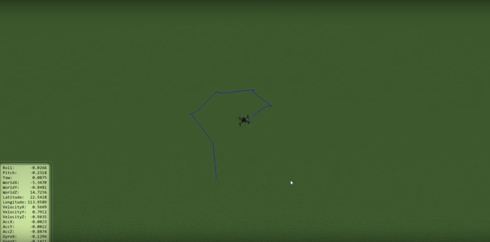
Figure 1. Screenshot for GPS waypoint following simulation
GPS Mission in DJI Assistant Simulator
February 21, 2020 – Pointcloud generation
Today we finish calibrating our depth cameras using the official application and were able to generate disparity maps and pointcloud.
However, due to limited bandwidth, we were unable to display all five disparity images at the same time. Thus, we are thinking of sending just the greyscale image, and leave future processing jobs to the onboard computer. In addition, the quality of the pointcloud is rather poor, so we need to find a different way for calibration in the future. We have also started working on simulation, we started by creating a mesh model of the drone in Gazebo. The next would be linking Gazebo with the official simulator.
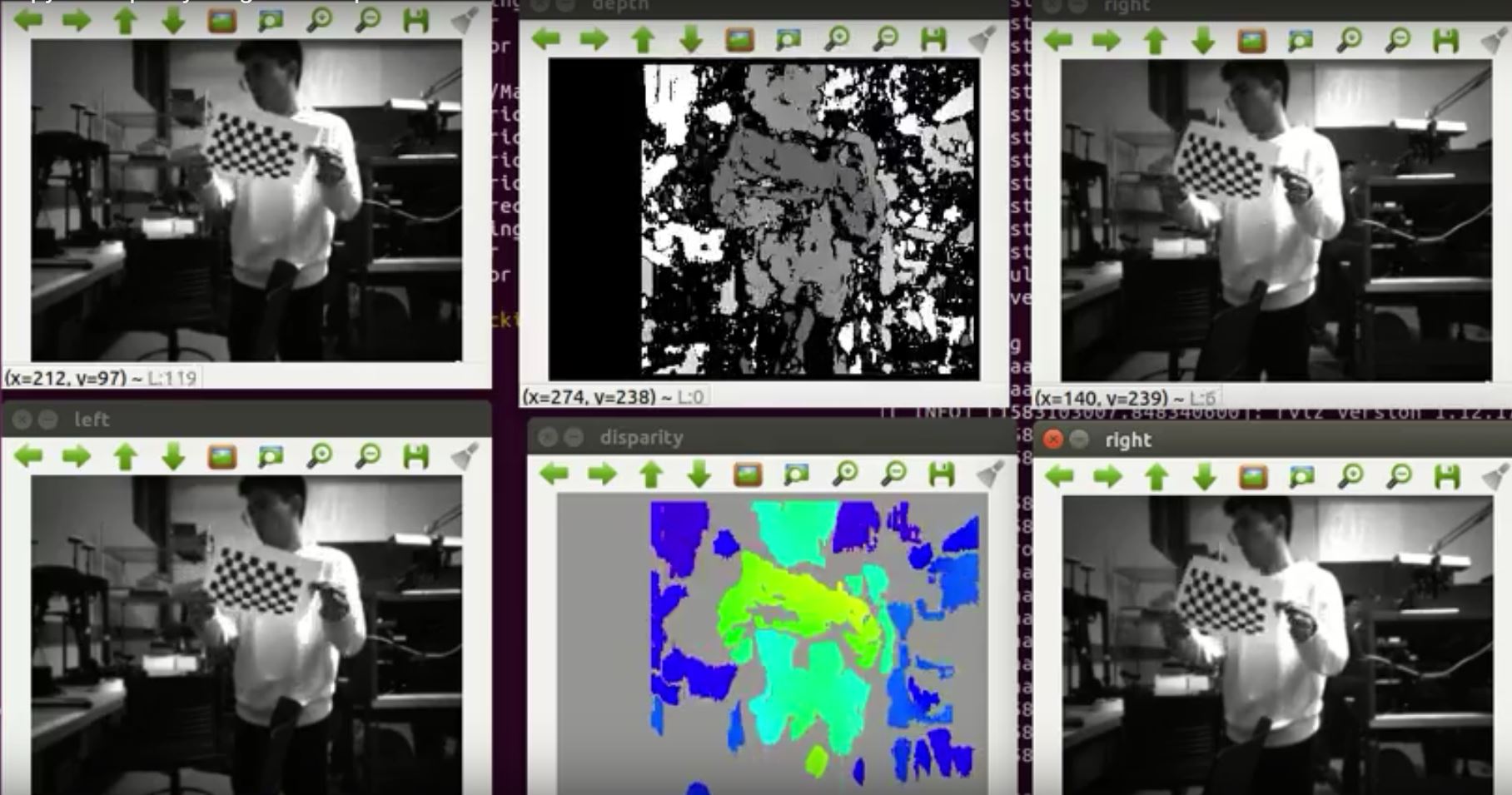
Figure 3. Disparity maps

Figure 4. Pointcloud generation
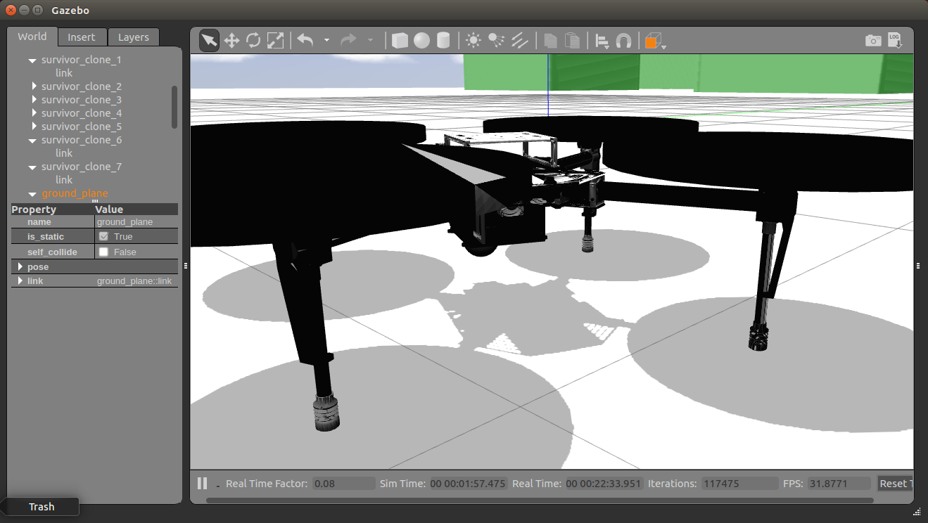
Figure 5. UAV model in Gazebo
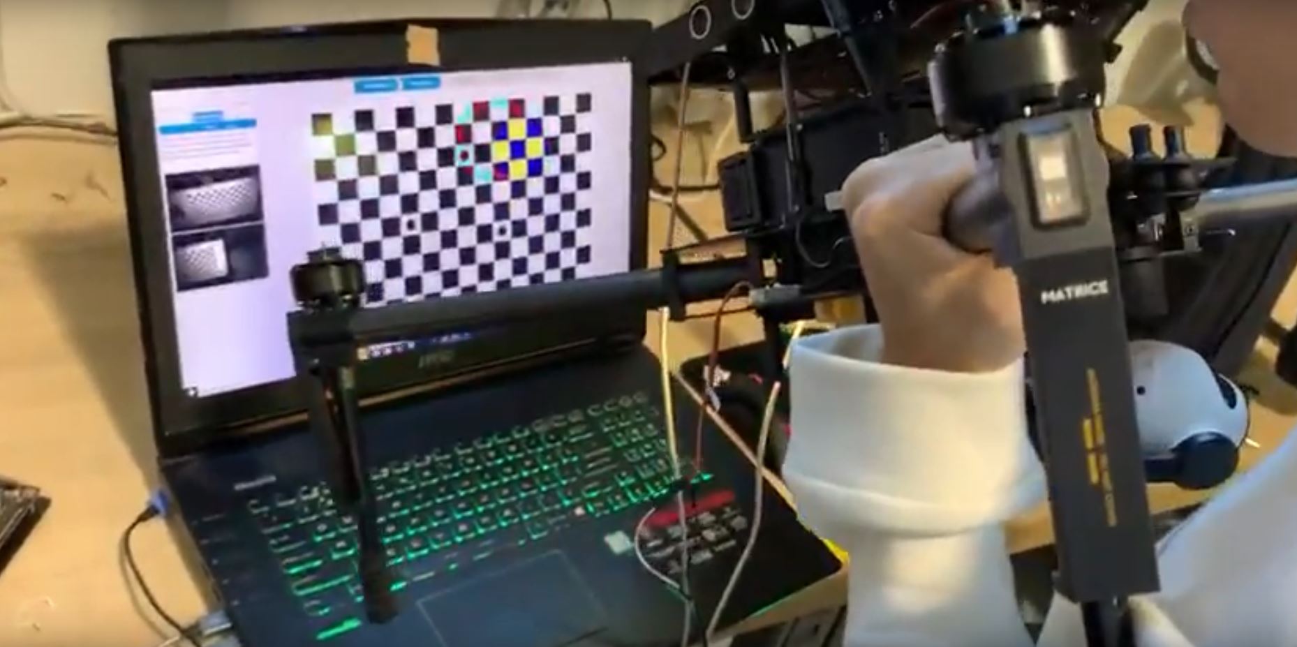
Figure 6. Calibration the Depth Camera
March 4, 2020 – Onboard Computer set up
Today we finished setting up our onboard computer for the UAV.
There were four major steps I took to set up the onboard computer: configuring the power supply, assemble the computer to a smaller extension board, reflash and set up ROS/Linux environment. The default output voltage from the drone battery is 22 V, which is too high for our onboard computer (19V max for Nvidia TX2). This was solved by purchasing a step-down converter online. In addition, the default carrier/extension board for the onboard computer is too big to fit on our UAV platform. The majority of its ports were extraneous and unnecessary for our project. Therefore, we purchase a much smaller third-party carrier board online with just HDMI, wifi and USB ports. The new carrier board is not compatible with the default setting of Nvidia TX2, so I had to re-flash it manually to be able to access the USB port. The final step was to set up a ROS/Linux environment similar to that of the laptop we have been used for running simulation. By following these steps I was able to run a similar GPS waypoint following demo that we showed during the last ILR with the onboard computer using the UAV battery as the power source.
Lastly, I was able to fit every component in an enclosure and mounted on top of the UAV. Specifically, I bought a third-party enclosure for the TX2 computer and the extension board. Then, I stuck the voltage converter onto the side of the enclosure using hook and loop. Lastly, I reorganized the components to clear a space at the top of the UAV where I fixed the entire module using hook and loop. This completes the hardware setup for the UAV except for the landing gear extension, and we should be ready for a test flight in full-autonomous mode for a GPS waypoint following the mission.
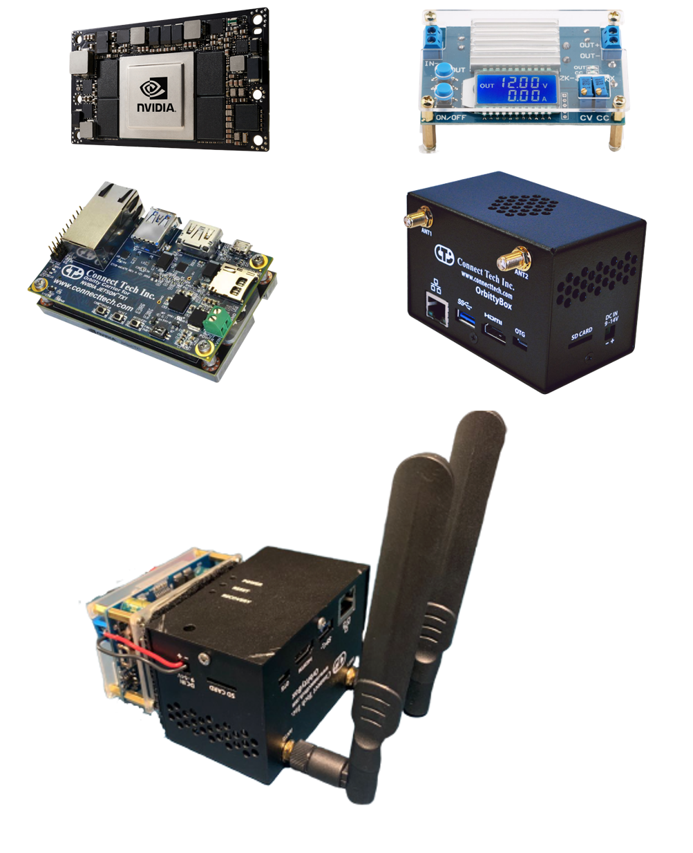
Figure 7. Components for the onboard computer and the computer after final installation
(From top left, Nvidia TX2, voltage converter, mini-sized extension board, enclosure)
March 17, 2020 – Re-work on point cloud generation
As I mentioned earlier, the quality of the point cloud we generated earlier wasn’t good enough for navigation. Thus, I was able to re-do the calibration using a different package with additional filtering. In addition, I also specified the relative position between the cameras and the base of the robot using the tf package.
There were three steps I took on processing it so that it can be fed into the path planner for obstacle detection. First, I decided to recalibrate the camera using a much larger checkerboard, as the point cloud quality under the previous parameter settings was not sufficient for capturing obstacles that are too small or too close. A comparison between the pointcloud using the old parameters and the pointcloud using the updated ones are shown below. Second, I also tuned parameters used by the block matching algorithms which transforms the stereo images to pointcloud. These parameters are responsible for different phases for the algorithm including pre-filtering which enhances the texture and normalize brightness, correspondence search along the epipolar line and post-filtering to eliminate bad filtering matches. The general goal for tuning is to capture the essential details for obstacles within a certain range and eliminate outliers as much as possible on top of that. Third, I specified the relative transformation between frames for each depth camera and the robot’s base frame. Using the tf package in ROS, I was able to use quaternion to define the orientation of each camera (front, back, left, right and bottom) with respect to the center of the robot. As a result, I was able to visualize all of them in the same frame in real-time. With these three steps taken, the pointcloud was ready to be used as input for a path planning algorithm.
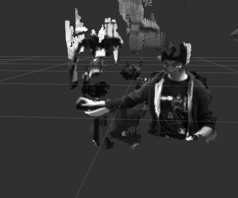
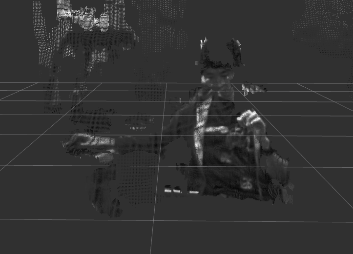
Figure 8. Pointcloud generated using old parameters (right) and updated parameters (left)

Figure 9. Pointcloud visualization in Rviz
Video for pointcloud visualization in Rviz
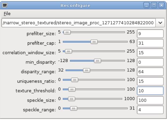
Figure 10. Parameters for the block matching algorithm
March 20, 2020 – Apriltag Tracking
Today we tested our Aprialtag detection and pose estimation algorithm. The idea here is to have a tag on the landing platform so we can use it for pose estimation during landing.
For the April tag tracking, I was able to recognize and publish the relative position relationship between the tag and the camera in real-time, which is similar to what we did for the programming familiarization assignment. The idea here is to have a tag on the landing platform so we can use it for pose estimation during landing. For future works, No.1 we will be controlling the movements pf the gimbal camera using this transformation data to track the tag. And No.2 we plan to increase the accuracy by using a cluster of tags instead of just one tag.

Figure 11. Apriltag tracking in rviz
March 24, 2020 – Simulation in Gazebo
Today we were able to simulate the UAV in a Gazebo environment side by side with the official simulator. The pose data of the UAV is sent from a pipeline between the UAV sdk and the simulator.
Creating the Gazebo simulation for the UAV was the most difficult work. It is because I not only have to understand the function of each API functions in the DJI official ROS SDK so we could control the motion of the drone by utilizing those functions but also need to convert the coordinate frame from the DJI Aircraft, which uses NED ground reference frame, to the Gazebo, which uses ENU ground reference frame. In the meantime, the DJI PC simulator automatically sets the initial take-off location as the reference point while Gazebo cannot do that. Without the initial take-off location being set as the reference point, the position of the UAV in the Gazebo world would make no sense. Therefore, I created a function to set the reference point in the Gazebo which is exactly the same as what the DJI PC simulator does.
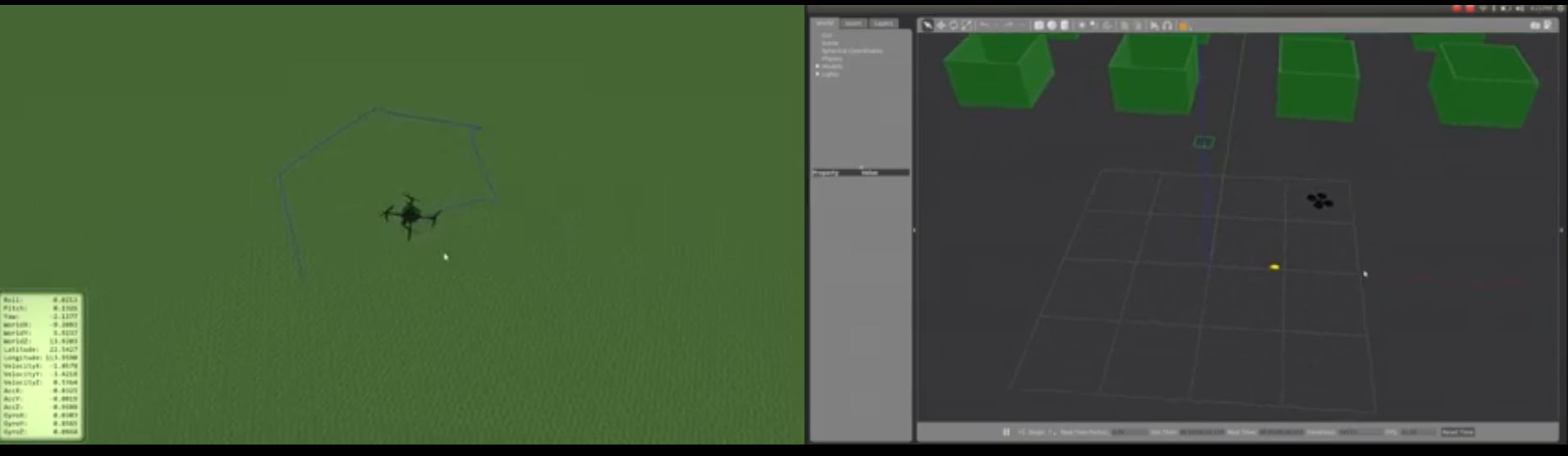
Figure 12. UAV running in the official simulator (left) vs in Gazebo (right)
Video of Gazebo GPS waypoint simulation
April 1, 2020 – Simulating Depth Camera in Gazebo
Today we were able to simulate the depth camera model inside Gazebo. We adjust the parameters of the fake camera based on the parameters or the real camera (intrinsic matrix, distortion parameters etc.). In addition, we were able to add a node of transferring the /pointcloud data to /laserscan data. We are doing this because most of the mapping packages online requires an input in the form of laser. As the figure shows below, we are able to visualize a pointcloud of a wall in the virtual environment as well as the laserscan topic transformed by the node (the white horizontal line).
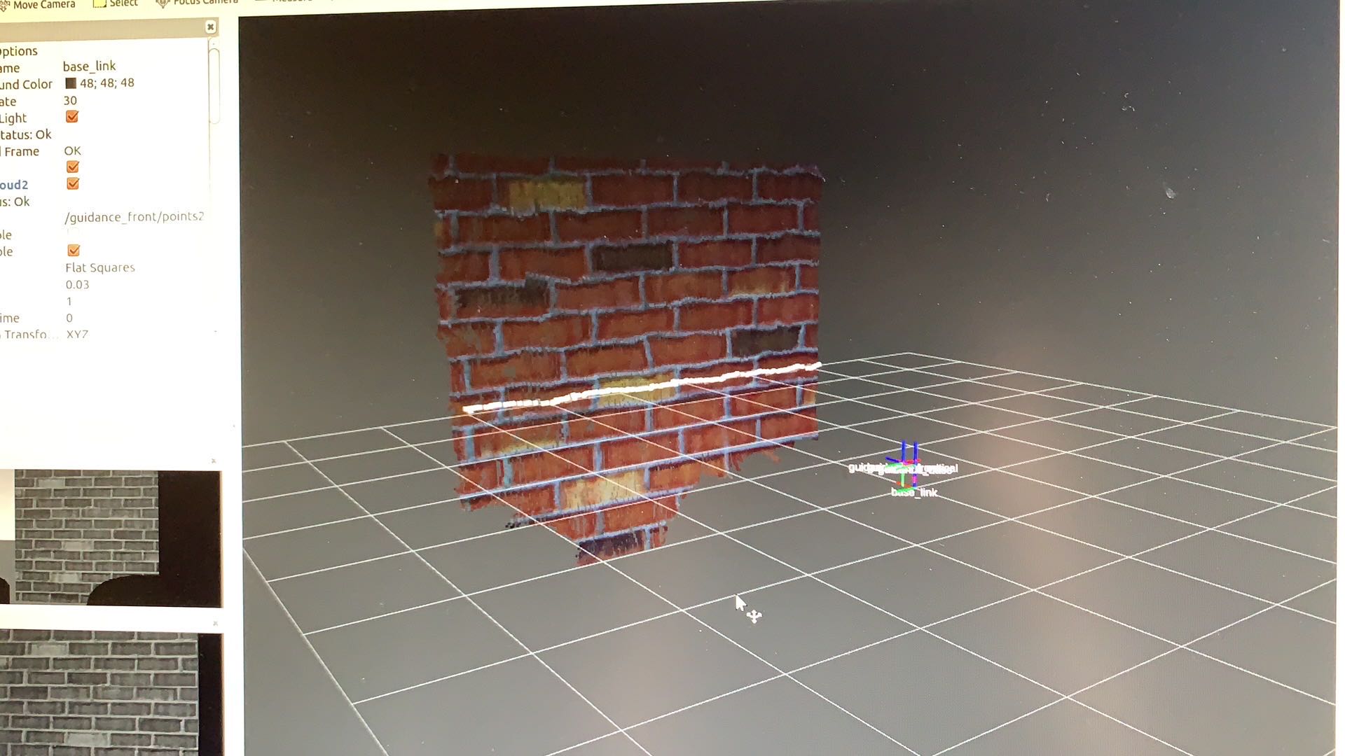
Figure 13. The pointcloud and laserscan generated in the simulation environment
April 8, 2020 – Laserscan 2D Mapping
Today we were able to finish implementing our 2D mapping module using gmapping. For the sake of simplicity, I decided to separate the mapping and localization for now. In addition, I decided to build a 2D map instead of 3D due to the computational constraint on the onboard computer and our functionality requirements. Specifically, I started out by using the point cloud generated by the depth camera and the ROS mapping package gmapping. Since gmapping is a laser-based package, I had to convert the 3D point cloud into 2D laserscan using a package called “pointcloud_to_laser_scan”. The result is shown below in Figure 14.
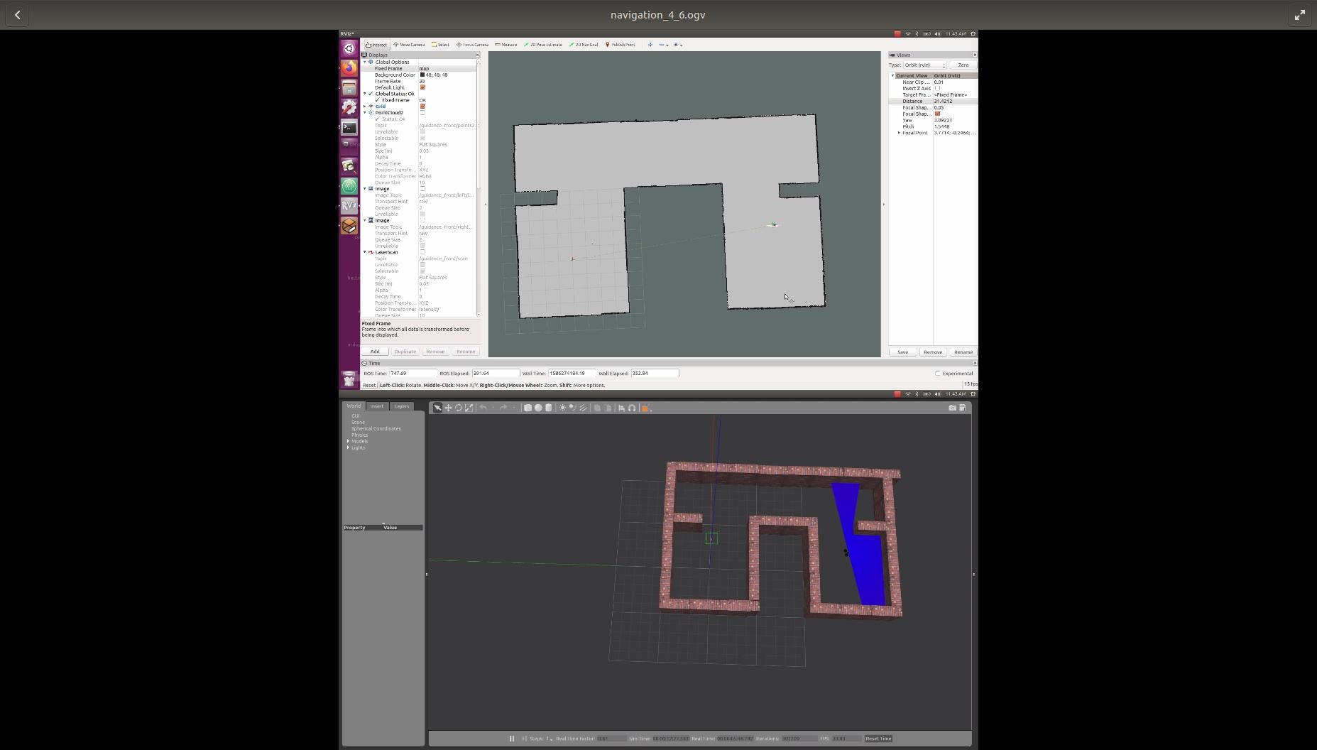
Figure 14. 2D mapping using laserscan messages with gmapping
April 14, 2020 – Navigation and obstacle avoidance
Today we were able to test out our navigation algorithm in Gazebo simulation. The UAV is able to follow the path specified by waypoints while avoiding simple obstacles. Although we implemented a mapping module earlier, we decided not to rely on any static maps or SLAM since this is not the focus of our project. We used a ROS package called “navigation” form the backbone of this module; it takes in information from odometry and sensor streams and outputs velocity commands to send to the UAV. Please see our SVD video for more details.
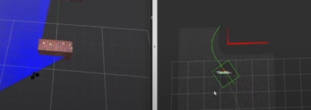
Figure 15. Rviz visualization of UAV path planning, cost map and obstacles
April 16, 2020 – Apriltag Tracking and landing
Today we finished our tracking and landing module, which allows the UAV to detect an Apriltag or tag bundle, measure its pose relative to base_link, and lands on the tag. We used apriltag_ros to implementing the tracking module with input from the right camera of the downward-facing depth camera. The detecting node we able to detect the tag from the greyscale video stream and output a pose transformation between the UAV and the tag in tf message type. The landing module is implemented using a PID controller which takes in position error between the center the tag and the UAV and output velocity control effort in row, pitch and yaw to the UAV’s motors. Please see our SVD videos for more details.
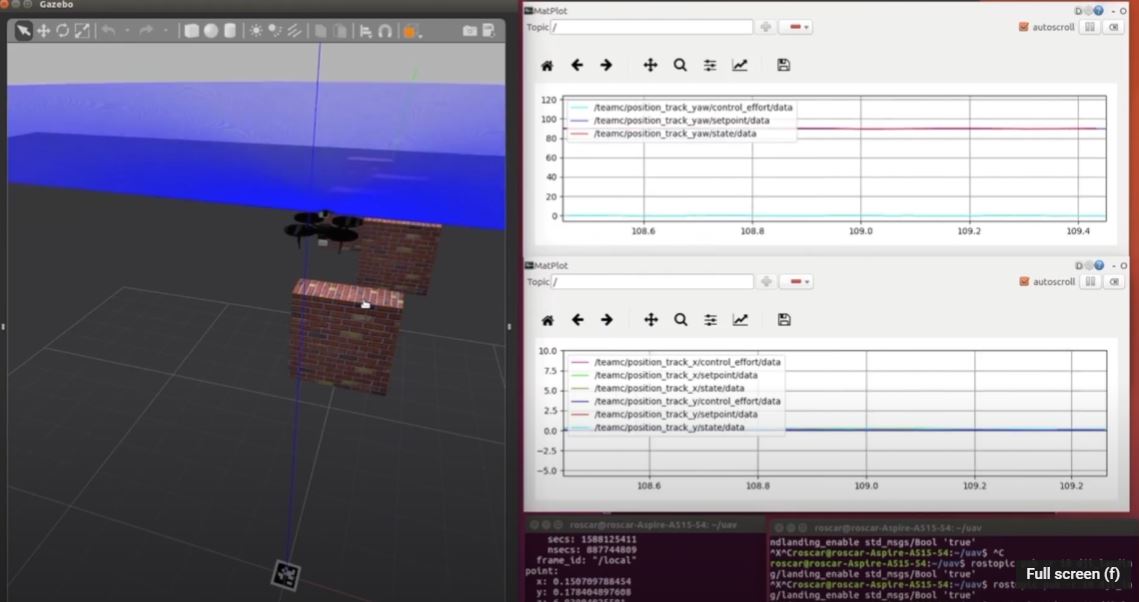
Figure 16. Rviz visualization of Landing process in Gazebo and PID control graphs
Sep 17, 2020 – Replace Depth Camera Set
The UAV was originally equipped with a visual sensing system, which contains 5 pairs of the depth camera. We planned to use the depth camera sets to do the Apriltag tracking and landing for the UAV. However, we found out that the software package of the visual sensing system developed by DJI cannot work on the NVIDIA Jetson TX2 on-board computer because the software package cannot support the ARM64 architecture. Due to the fact that the software package is no longer maintained by the DJI, we could not get a software package of the visual sensing system which supports the ARM64. Therefore, we immediately replaced the depth camera sets with one monocular camera for Apriltag tracking and one 2D laser scanner for obstacle avoidance. The pictures below show the monocular camera and 2D laser scanner.
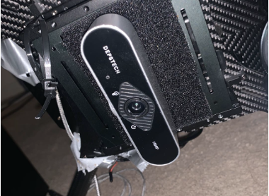
Figure 17. Monocular Camera
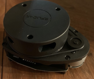
Figure 18. RPLidar 2D laser Scan
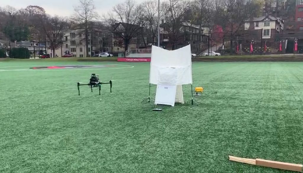
Sep 30, 2020 – Field-testing for Apriltag Tracking and Landing
We started to perform the UAV Apriltag tracking and landing field test in the Boyce Park. Fig.19 shows the hardware preparation before the test. The UAV is equipped with the propeller guard and all the sensors are mounted on the UAV. We put a big Apriltag on the ground for the UAV to track and land. The Fig.20 shows the Rviz visualization for the downward-facing webcam and tag detection. As shown in the image, the webcam works normally and the UAV can successfully detect the Apriltag in the outdoor environment.
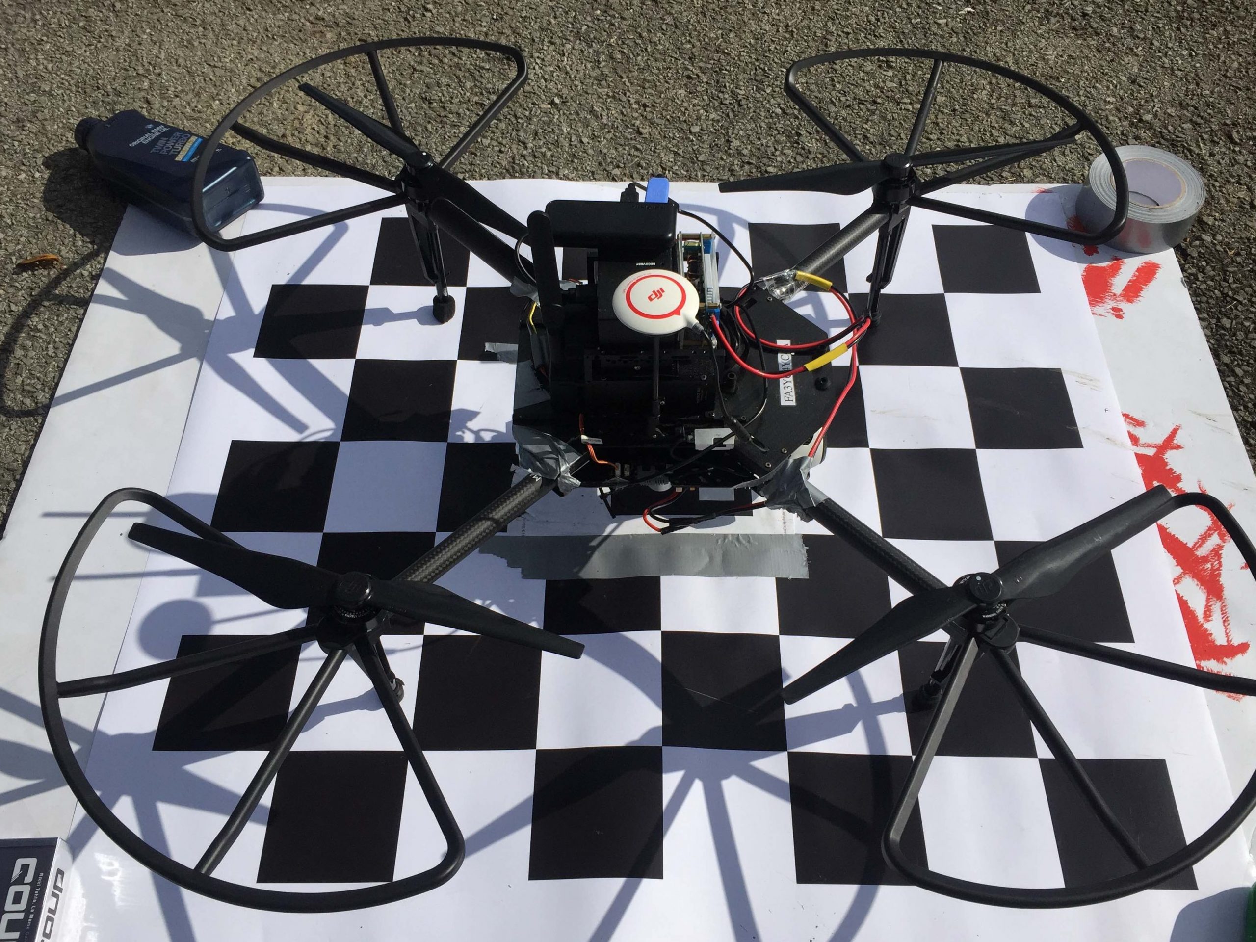
Figure 19. UAV hardware setting before field-testing
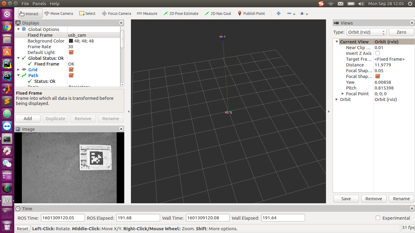
Figure 20. Apriltag detection visualized in Rviz
The overall procedure of the landing is to first manually take off and flies the UAV on the top of the tag and then let the landing algorithm take over. The UAV keeps measuring the X-Y position error between the UAV current location and the tag location while flying towards the tag horizontally. The UAV will start descending until the position error is below a certain threshold. During the Apriltag tracking and landing, the PID controller is used to generate the control effort for the UAV to minimize the position error. The overall algorithm works perfectly in the Gazebo simulation, though, the UAV was barely going down during the actual field test. This is because the weather was pretty windy during the field test and the control effort limit for the PID controller was too small for the UAV to fight against the wind. We expect to solve this issue and let the UAV land stably by increasing the control effort limit for the PID controller.
Oct 14, 2020 – Field-testing for Navigation
First of all, we were able to set up the 2D laser scanner we purchased previously, which is crucial for the obstacle avoidance ability. We installed the laser scanner on the top of the UAV with a 3D printed base using screws. Then we developed the software package and added the tf transformation for the laser scanner to detect obstacles and send the correct laserscan message relative to the body frame. Fig. 21 shows the visualization of the obstacle detection by laser scanner in Rviz.
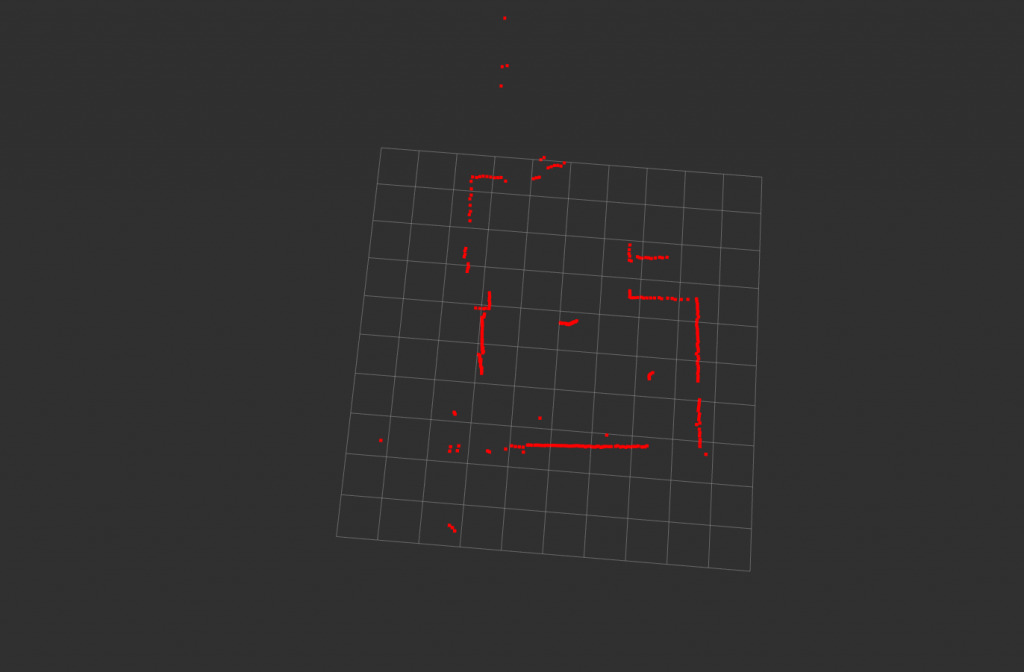
Figure 21. Laser scan visualization in Rviz
For the navigation field-test, we placed one card box on the ground about 5 meters away from the UAV as an obstacle. We let the UAV autonomously take off and then let the navigation algorithm take over. In the meantime, we manually assign several waypoints via Rviz to test whether UAV could fly to the waypoint while avoiding the card box. During the test, we intentionally set a waypoint that is too close to the obstacle and the UAV can identify this waypoint is an invalid point instead of crushing onto the obstacle. With a valid waypoint set behind the obstacle, the UAV was able to plan a path around the obstacle under the safe distance constraint.
Oct 29, 2020 – Field-testing for Landing
To increase the accuracy of the landing, we added a smaller Apriltag beside the bigger one. UAV can also detect the smaller Apriltag when its height is too low such that the landing would be more accurate. We also drew a circle on the platform to denote the landing receptor installed on the UGV.
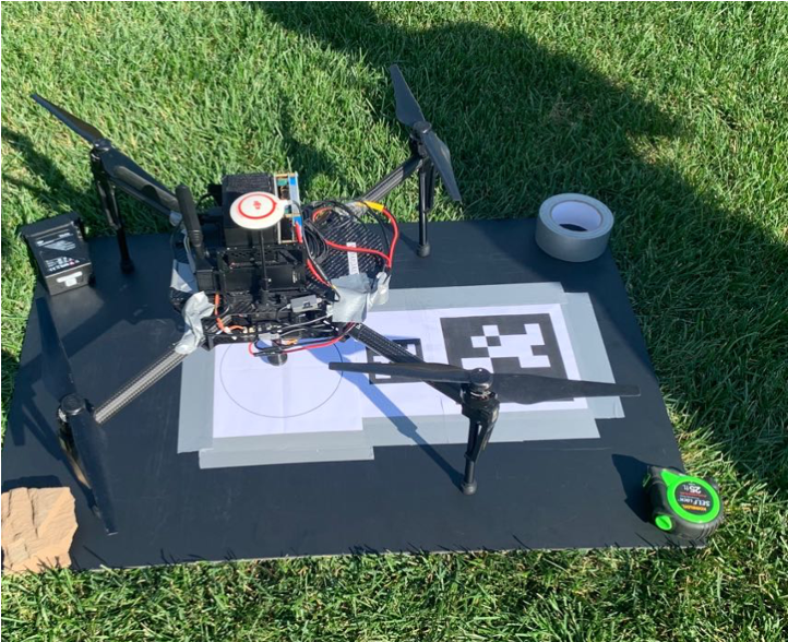
Figure 22. UAV successfully lands on the Apriltag
Nov 11, 2020 – Integrated Landing Test
We tested the UAV landing onto the integrated landing platform. The test setup is shown in Fig.23. The landing process is vision-based, with two April-tags in different sizes, for guidance in different height levels. The paperboard platform serves as a protection purpose to prevent the UAV from falling. The UAV landing module will eventually insert into the receptor after a successful landing trail.
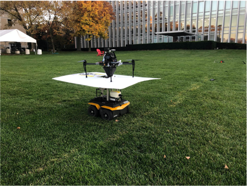
Figure 23. Landing with integrated landing platform
Nov 14, 2020 – Integrated Landing Test
We tested the navigation field test with actual GPS coordinates. For previous tests, we have been assigning goals in the local odometry frame to the UAV rather than with latitudes and longitudes in the global frame. And since the navigation stack uses cost maps in the local frame, we had to write a function converging the coordinates from ground frame to local frame using the haversine formula, which calculates the great-circle distance between two points. We then field-tested our implementation over the Mall using a landmark with known GPS coordinates gathered from Google Map. The results were quite successful: the UAV was able to reach the landmark with a positional error of fewer than 2 meters.
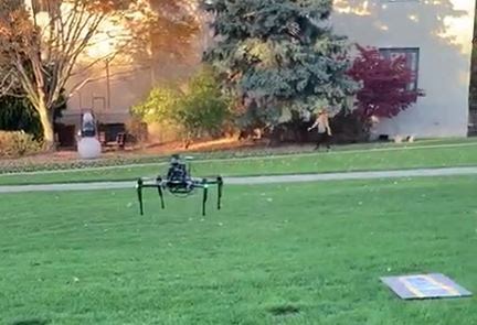
Figure 24. UAV navigates to the tag with GPS guidance
Nov 18, 2020 – FVD Rehersal
Today we performed a dressed rehersal for our FVD, including waypoint following with obstacle aovidance as well as landing on top of the UAV.