Fall Semester Implementation Details (Final Version)
Any autonomous car is required to adhere to the rules of the road, namely staying safely within the desired lane. We wanted our system to follow these rules as well. In order for our lane following functionality to work, we had to make one assumption about the garage environment. We assumed
there to be a solid line dividing the two lanes within the garage, which we saw in our testing environment in the CMU East Parking Garage. We performed lane detection to segment the lane in camera images obtained from the d435. This information is later used in the goal generation and
navigation stage.
At this point, we have decided to switch from deep learning neuron networks to classical computer vision methods for both hardware and simulation. It turns out that it worked pretty fine in both cases.
We utilized classical computer vision methods to detect the center line in the lanes. We had initially been pursuing deep-learning-based methods for lane detection in the spring semester. However, we abandoned that method due to insufficient labeled data for training the system to work in the physical parking lot, as well as the fact that the training we performed on simulation data did not translate well to the physical environment. To make sure our subsystem is robust, we manually place a yellow seat belt on top of the center line in the CMU parking lot, since the existing road paint was fading. Our lane detection algorithm is described in five steps, summarized below.
1. Perform HLS thresholding on a region of interest in the bottom-left of the image in order to
filter out the yellow seat belt
2. Detect the line using a Canny edge detector and probabilistic Hough transforms.
3. Project the pixels on the line into a 3D point cloud using the depth camera
4. Find the normal vector of this new linear point cloud using singular value decomposition (SVD)
5. Generate the right boundary line by extending mirroring the current point cloud along with a pre-determined lane width.
The point cloud of the center line and the right lane boundary is sent to the navigation subsystem as an obstacle constraint in the costmap. We also generated an ego-line point cloud by extending the center line point cloud to the right with 60% of the lane width. This ego-line point cloud is later
sent to the goal generation subsystem as an input, and goals are generated along this line. Overall, the lane detection subsystem is crucial to the success of the whole pipeline since both the goal generation and navigation subsystems rely heavily on accurate lane detections.
Spring Semester Implementation Details
The purpose of the detection subsystem is to identify lanes in the environment in order to impose a constraint on where the robot can move. As of now, this system is still in progress, as we have been trying several different methods for lane detection with varying results.
Hardware
Progress up to Progress Review 9
We are using classical computer vision methods here. The reason we gave up leveraging deep learning techniques to detect lanes in real-world data was because of insufficient labeled data for training. Moreover, the model trained in the simulation could not be transitioned to the real world properly.
To make sure our subsystem is robust enough, we manually place a yellow seat belt on top of the faded center line in the CMU parking lot. Our lane detection pipeline in hardware could be decomposed into the followings:
- HLS thresholding with the image in order to filter out the yellow seat belt.
- Detect the line with
opencvfunctions such asCanny()andHoughLinesP(), as shown in Fig. 1 & 2. - Project the pixels on the line back to the 3D world with respect to the depth camera.
- Find the normal vector of the line using SVD.
- Interpolate the right line by extending each point cloud with a fixed lane width, as shown in FIg. 3.
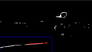
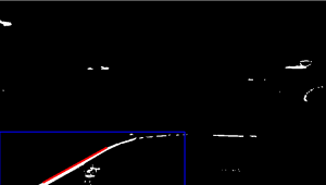
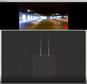
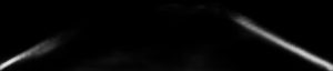
Fig.3 Lane Projection
Simulation
Milestone For SVD
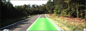
Before the spring semester ends, we had our detection system successfully running under simulation. Our final decision is to use a deep network to get a segmented lane output. We use the ERFNet model, as shown in Fig.4, which was initially trained to segment detect lane lines in a highway scenario. We realized we had to collect custom data in the simulator and retrain part of the network. We have designed an automatic data collection pipeline in the simulator, as shown in Fig.5. To illustrate, we collect both data and label images simultaneously by tele-operating Husky around in the parking lot. The way we do this is that we first color the right lane of the ground image light green, and while tele-operating Husky around, we take the RGB image of the front camera and process it into data and label images. To recover the original data image, we replace the green pixels with gray. To get the ground truth label image, we replace the green pixels with pixel value 255 and all the other pixels with pixel value 0. This way, we make sure the time stamps between the data and the label are consistent.
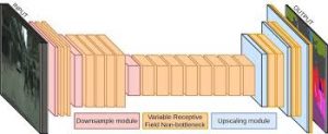
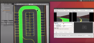
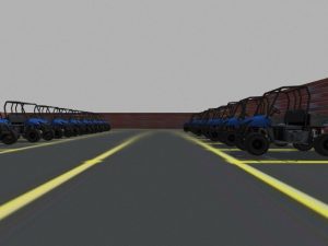
Fig. 4 ERFNet Model Fig. 5 Screenshot During Data Collection

Fig. 6 Lane Detection Outputs in Different Views
Prior Work
Our first attempt to solve this problem utilized classical methods of computer vision to find lines and perform polynomial fitting over the lines found in the image. This produced solid results when tested on the KITTI dataset. When testing on our simulated parking lot, this algorithm had some issues dealing with sharp turns, specifically the fact that both lane lines may not be visible at all times during a 90-degree turn. Below are test images of this method on the KITTI dataset and on our Gazebo world.