
Project Implementation Details
Overall System Description
Our main objective is to enable the chassis to autonomously dock and undock with a modular pod and navigate in a geofenced environment. The required inputs to the system are energy (battery power) and information (such as a precomputed map of the operating environment and the user request). Based on this input and the state of the system, it performs point-to-point (P2P) navigation, approach navigation, docking, and undocking, while ensuring safety by continuously monitoring system health. The overall functioning of the system is determined by the state machine transitions, as shown in Figure 1.
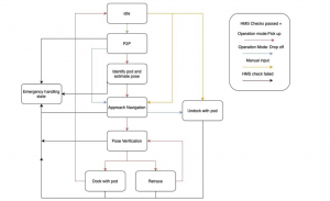
Figure 1: State machine diagram representing our overall system.
1. Sensing Subsystem
Hardware
Spring Semester Status
We are in the process of assembling the PIXBot that has been shipped to us. We had to get the tires fitted to the rims, and then fit the wheels onto the main chassis. The next step was to open the chassis up so the battery can be mounted onto it. The assembled chassis with the wheels attached is shown in Figure 2.
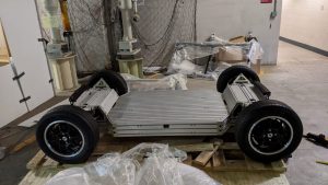
Figure 2: Assembled PIXBot chassis.
Fall Semester Updates
We faced several issues with getting the PIXBot hardware up and running, including a battery pack, shown in Figure 3, that refused to stay charged, possibly as a result of being dormant for several months due to the pandemic. We opened up this battery pack and analyzed the voltage at various terminals (and also disconnected and reconnected them to force a system reset for the Battery Management System), but unfortunately we were unable to salvage it.
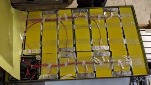
Figure 3: Disassembled battery pack
For the purposes of our demonstrations and for testing our algorithms, we designed a makeshift setup (shown in Figure 4) involving the full set of sensors (camera, 2D LiDAR and 3D LiDAR) from PIX Moving mounted on a movable cart platform.
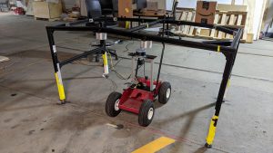
Figure 4: Moving cart hardware setup
Perception
Spring Semester Status
We focused on using the camera data with an existing YOLO pipeline for frame-by-frame prediction of various obstacles. We also used the 2D LiDAR data and checked all obstacles within a narrow field of view, and used this to inform the Health Monitoring System in case the threshold of minimum detection had been reached. We also tried to use Autoware features like point cloud clustering and L-shaped matching, but did not use this to inform any of the other subsystems.
Fall Semester Updates
We are detecting and tracking pedestrians by fusing detections from the camera and the LiDAR on the vehicle. There are two streams of data that are combined here. The first is from the camera. The images are fed into a modified YOLO network, which detects pedestrians only (as per our current use case). These detections are fed into a DeepSort tracking system, which uses features of the pedestrians to assign them an identity and track them. The output of this stream is a bounding box for each detected pedestrian and a unique number that is associated with their identity. The other stream is LiDAR information. We use Autoware’s point cloud clustering and L-shaped matching algorithms to extract cluster centroids of detected objects. These cluster centers are then projected onto the image. The projections are mapped one-to-one to find correspondences between the pedestrian bounding boxes and the clusters. If the cluster is not related to a bounding box, it is labeled as a miscellaneous obstacle.
These detections are then converted into a color-coded bird’s eye view image for visualization, which can then be passed onto the prediction pipeline. Figure 5 shows the demo of the system in the simulation, and also shows the 2D laser which is used as a redundant obstacle detection sensor.
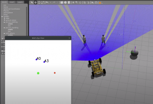
Figure 5: Bird’s Eye View result with Pedestrian Tracking.
2. Navigation Subsystem
Spring Semester Status
We also obtained the intrinsics of the Mindvision camera using the ROS camera calibration utility, and then implemented trajectory tracking and pose estimation using AprilTag markers as ground truth poses (shown in Figure 6).
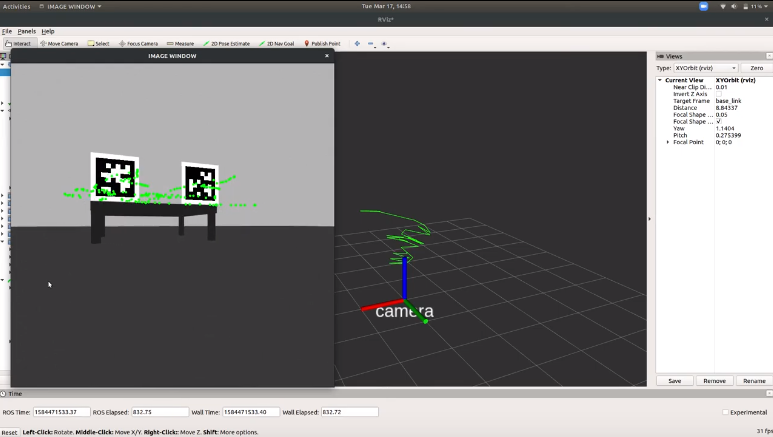
Figure 6: Trajectory and pose tracking using AprilTag markers for ground truth
The alignment sub-block in the navigation subsystem involves the relative localization of the chassis relative to the pod when in the Payload Handling Zone (PHZ), and then generating and executing a path from the entry point of the PHZ to the goal location under the pod (approach navigation). We built a simulation (described further in the simulation subsystem) that uses a 2D LIDAR in conjunction with the AprilTag markers for the purpose of relative localization of the chassis with respect to the legs of the pod, when it is in the PHZ.
We also explored a few different methods for approach navigation, including:
- deep reinforcement learning for trajectory generation (following this paper for the unicycle model and then implementing the same for an Ackermann steering model using OpenAI_ROS)
- trajectory optimization using quintic Bezier curves
- trajectory generation using Dubin’s Curves.
We implemented the RL model using a custom OpenAI Gym environment, and also verified the other two using a custom ROS+Gazebo setup with a model of an Ackermann vehicle. We later obtained the CAD model of our chassis from PIX and used that in place of the model too. We finally decided to generate a set of waypoints with strict constraints on the allowed steering angles and velocities to perform the docking maneuver, and then followed these with pure pursuit and a PD controller.
The prediction sub-block of the navigation subsystem is currently in the research phase, and we have looked into Autoware’s “Beyond Pixel” based object tracker, as well as Probabilistic Graphical Models.
The mission planning sub-block of the navigation subsystem is responsible for global planning and trajectory/waypoint generation and we implemented this using the CARLA-Autoware Bridge and providing initial and final goal positions using RViz. This is shown below. We later switched this to waypoint following using pure pursuit in a Gazebo simulator, since CARLA was unstable. The vehicle is able to stop for obstacles along the path.
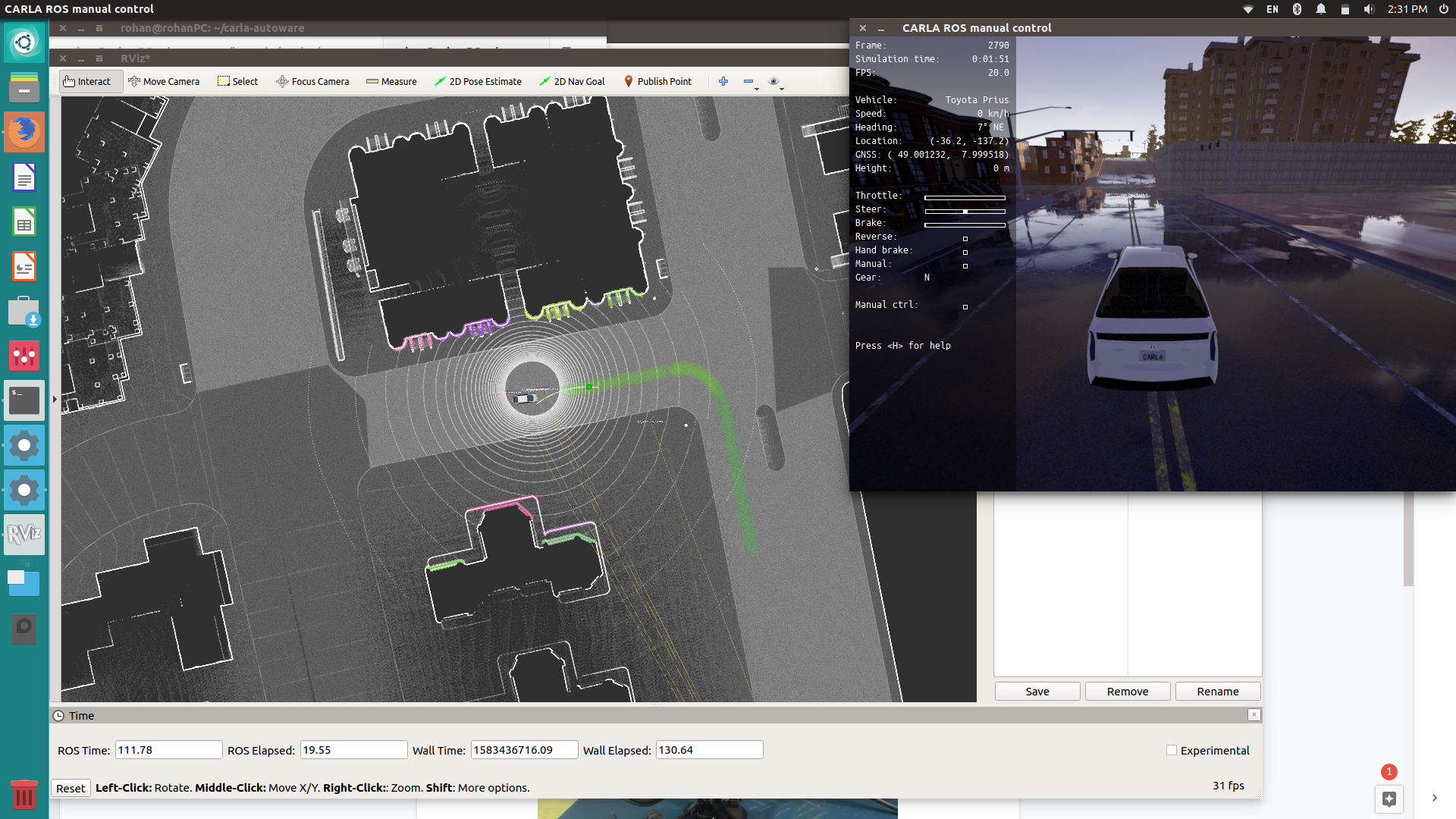
Figure 7: Point to Point Navigation in CARLA using the CARLA-Autoware Bridge over ROS
Fall Semester Updates
We completed detached our system from the CARLA software, and we shifted to using the ROS move_base package’s Timed Elastic Band (TEB) local planner and implemented custom global planners based on Reeds-Shepp and Dubins curves. Dubins curves do not allow reverse maneuvers, and so our retrace functionality would have been more complex, requiring a full 360 degree rotation to return to the original entry point of the docking zone, as shown below in Figure 8. However, Reeds-Shepp curves (shown in Figure 9) do support this reversing maneuver, and as a result, they can generate more realistic and optimal car-like paths for the retrace or further navigation tasks.
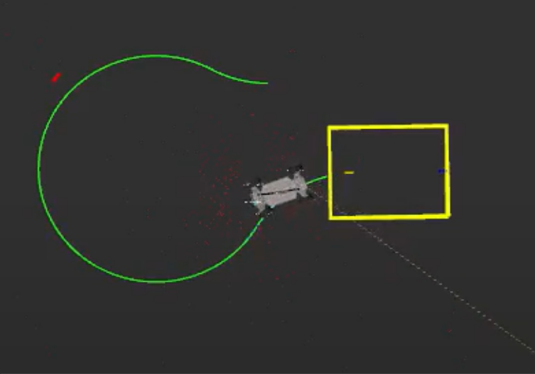
Figure 8: Dubin’s curves for “reverse” maneuvers – requires a full U-turn while always driving forwards
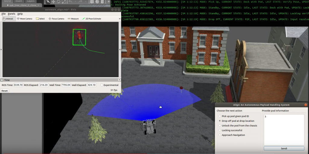
Figure 9: Reeds-Shepp curves allow for reversing from the docking zone and traverse to other locations, or perform a retrace and try docking again
The TEB local planner allowed us to specify a sparse set of waypoints (pose and location) from the starting location to the goal location where the docking/undocking had to take place, and the planner would generate a trajectory that interpolated optimally between the waypoints given a set of tunable parameters. We also used this to our advantage with the help of actionlib and asynchronous calls when implementing the obstacle detection subsystem, and we had the local planner automatically stop the execution of the current plan in case of an emergency, but then continue the execution once the hazard has been taken care of.
3. Docking Subsystem
Spring Semester Status
The docking position verification will be done by comparing the relative pose of the vehicle with respect to the pod once it has reached the docking position. We perform the docking procedure by predicting the location of the pod using the four legs visible in the range of the 2D LIDAR mounted on the front of the chassis. We then generate a set of five waypoints that plan a path from the current pose and orientation of the chassis to the desired goal pose under the pod. We have implemented strict constraints on the steering angle and velocity at each waypoint. We execute this path using standard pure pursuit with PD control of the velocity and the steering angle.
The path in RViz is shown below in Figure 10 (green arrows). The yellow rectangle is the prior estimate of the pod location, and the green rectangle is the estimated location of the pod generated from the 4 legs of the pod using the 2D LiDAR. This is continuously refined as the chassis moves under the pod. The docking verification is performed once the chassis has completely executed the path. It uses the 3D LiDAR data in a circular region around the sensor and averages it to get the location of the pod center. In case there is an error in the final docking, the system performs a retrace procedure, by going back along the waypoints and performing the docking once again.
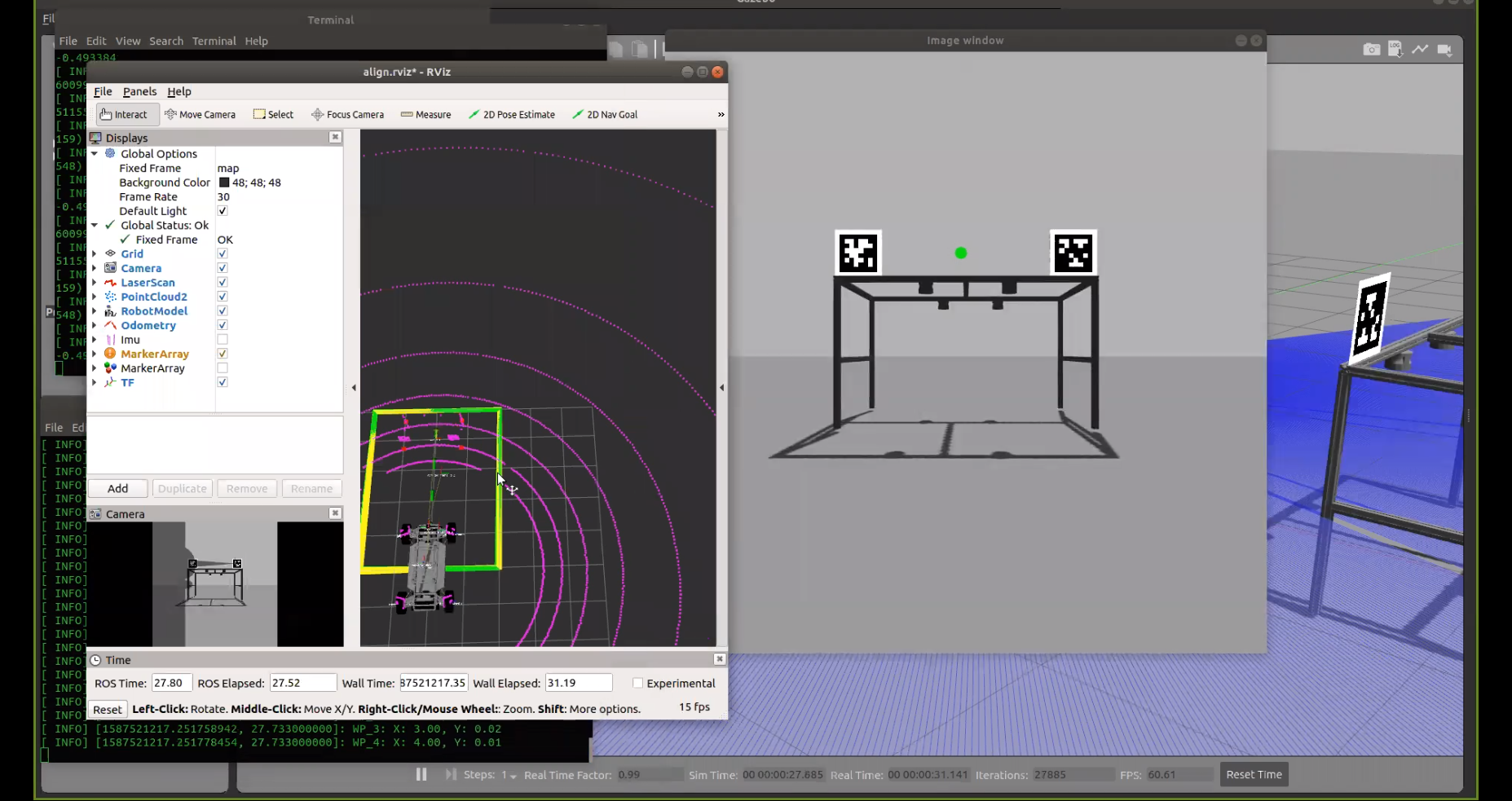
Figure 910 Generating Docking Pose estimate and Waypoints using 2D LIDAR
Fall Semester Updates
We implemented the docking actuation in simulation, through the use of prismatic joints and a PID controller to control the linear actuation that lifts up the pod. This is shown in figure 11.
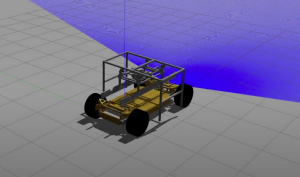
Figure 11: The pod being lifted up by the docking mechanism.
The docking verification algorithm was improved to remove the effects of clutter by considering cylindrical thresholds around each pod leg and then averaging these points to form an estimate of the pod leg center, and finally using these to get the center of the pod. The visualization of this is shown below in Figure 12.
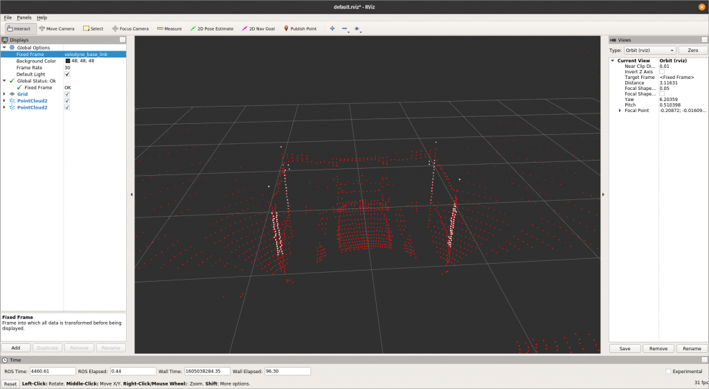
Figure 12: Docking verification visualization. White points correspond to points that are estimated to correspond to each pod leg, whereas the red points correspond to the point cloud from the 3D LiDAR.
4. Safety Subsystem
Spring Semester Status
- Health Monitoring: Our current implementation monitors the functioning of the obstacle avoidance node, 2D and 3D LiDAR sensors, and NDT pose information. The system is brought to a halt if an obstacle is detected, and information is logged about the node and the topics based on persistence and sanity checks of data received. This is shown in Figure 13.
- Emergency Handling: We command the vehicle to come to a halt in case of any inconsistencies in sensor data, or an obstacle crossing the path or if nodes crash. The command velocity is set to zero and this would be controlled through the PID controller for the motors to ensure the vehicle smoothly comes to a stop.
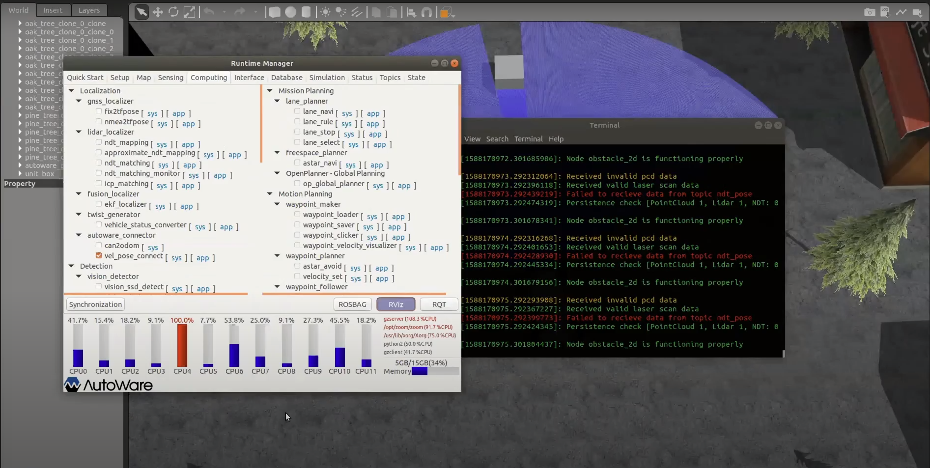
Figure 13: Health Monitoring System logs during NDT Matching failure
Fall Semester Updates
We integrated the Health Monitoring subsystem with a system-level state machine that ensures safe transitions between various states. We discussed this design over a team Zoom call (Figure 14), and a rough sketch is shown below. We also implemented a Graphical User Interface (GUI), described in the following section, that makes it easier to transition between various system states manually for demonstrating various functionalities. We designed different types of messages to pass this data around through the system, and we tested the stability of various state transitions algorithmically.
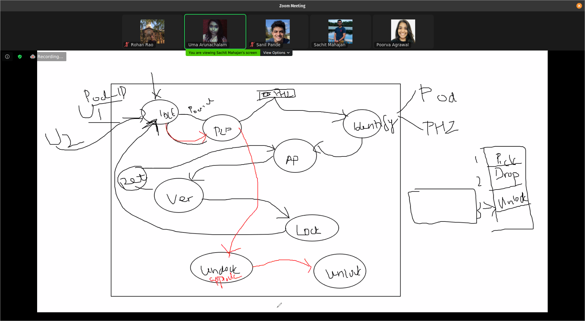
Figure 14: Brainstorming a state-machine design for the Health Monitoring subsystem
5. Simulation Subsystem
Spring Semester Status
We used the Gazebo simulation shown below to bring in our actual chassis model, test the low-level Ackermann steering and control with PID, integrate with a 2D LIDAR for relative localization with respect to pod legs, camera with custom intrinsics, AprilTags for relative pose estimation and trajectory tracking, and tele-operate or track trajectories generated based on reinforcement learning or splines. These are shown in Figure 15.
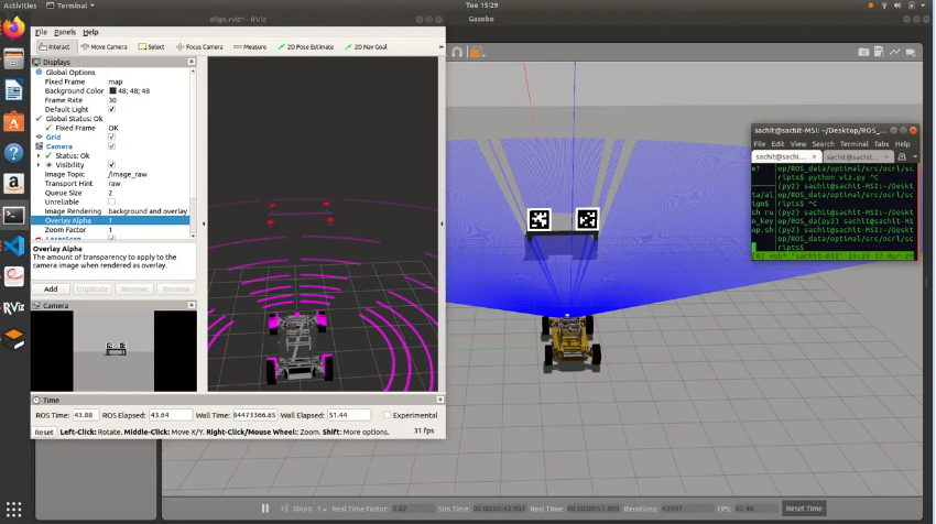
Figure 15: Gazebo+ROS Simulation environment for the chassis, with AprilTags, 2D LIDAR and camera
After analysis and testing within CARLA, we found that the point-to-point navigation within CARLA was unstable (it would crash often and was unrecoverable), and so we decided to shift our entire Autoware and Simulation pipeline into Gazebo. For this purpose, we used a custom Gazebo world that was provided by Autoware (Figure 16), along with the pre-computed point cloud map generated using NDT Mapping, and a set of waypoints for going around the entire map (Figure 17).
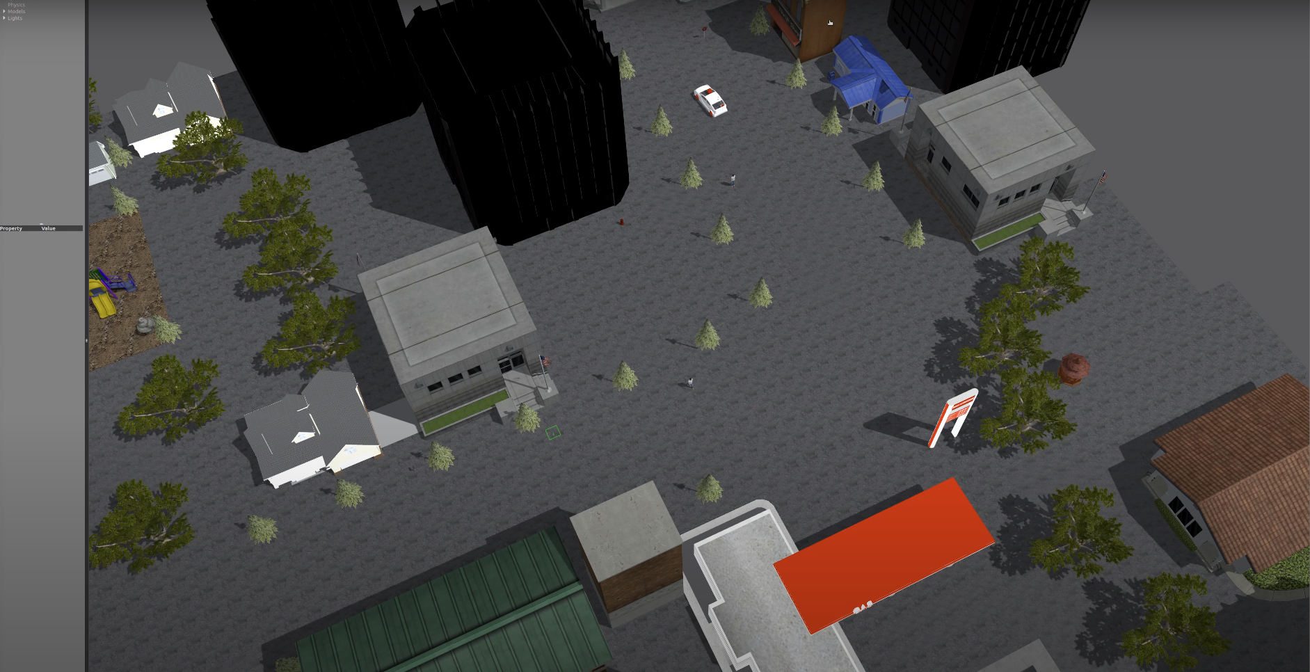
Figure 16: Autoware-Gazebo simulation for high-level navigation and planning
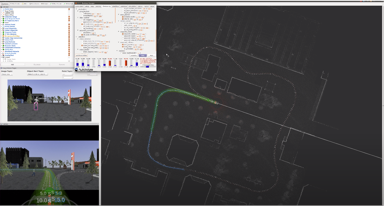
Figure 17: Autoware-Gazebo simulation showing map and waypoints
Fall Semester Status
For the Fall semester, we worked on merging the docking simulation shown in Figure 15 with the Autoware-Gazebo simulation shown in Figure 16. This enabled us to demonstrate all of our subsystems in a single integrated environment and also enabled us to add in multiple pods along with possible pickup/dropoff locations. Using the state machine enabled us to switch between all of the system’s states effectively so as to enable switching from P2P navigation to approach navigation.

Figure 18: GUI designed for quick inter-state operation and demonstration of functionality
We designed a GUI using Qt with which we could command the vehicle to go to a specific pod location to pick it up as well drop it off to the commanded location. We also added in commands to manually instruct it to unlock, to switch to approach navigation , or to signal to the state machine that locking was successful.