The System
Tool
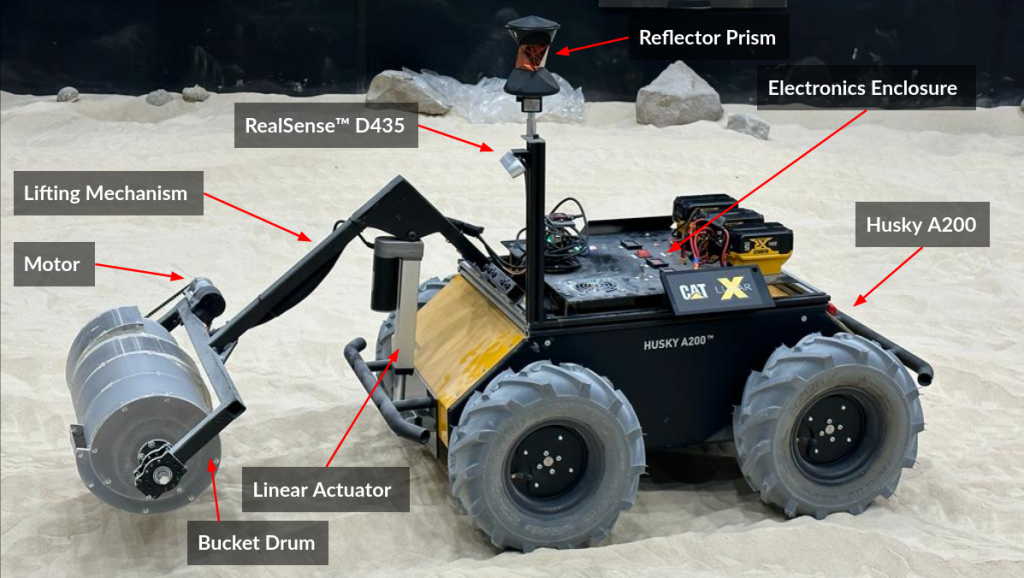
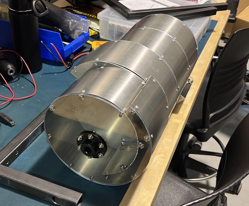
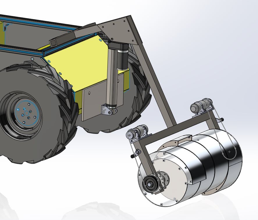
The tool is crucial for the system, consisting of two main components: the bucket drum and the lifting arm. The bucket drum is responsible for regolith-related operations such as excavation and deposition. Its unique design excavates material when rotated in one direction and deposits material when rotated in the opposite direction. The bucket drum is made up of four separate sections, each with a cutting edge phased out at 90 degrees to reduce the cutting force acting on the tool at any given moment. The bucket drum is driven by a belt and a 135 kg-cm, 60 RPM motor. The effective gear ratio of 2.25:1 increases the operational torque, providing an additional factor of safety.
The lifting arm is responsible for raising and lowering the bucket drum. It has been built to lift the bucket drum to 45 cm above the ground level and lower it to as low as 5 cm below ground level. This range of motion ensures the system can build a berm bigger than the minimum requirements while also being able to excavate in low-lying areas. The lifting mechanism is actuated using a linear actuator.
Electronics
The electronics architecture that powers the system has three sources for three different power circuits. These circuits are for powering the computer, the actuation, and the mobility separately. This separation ensures that the emergency button only cuts off the power to the mobility and actuation, leaving the compute and sensing subsystem unaffected.
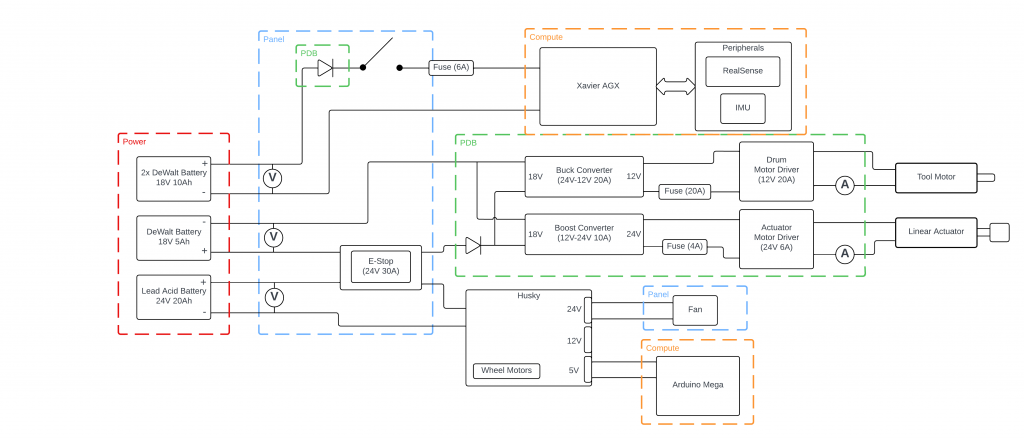
To maintain the safety of the system, there have been fuses installed wherever required. Voltmeters help in keeping the battery voltages in check during operation. There are two voltage converters to provide the appropriate voltage levels to the actuators. These actuators are controlled using the respective motor drivers. To help monitor the system conveniently, there are five status LEDs installed on the electronics panel of the system.
Software
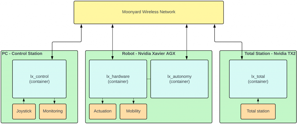
The software architecture onboard the system is divided into multiple modules. The majority of the components are implemented using the ROS 2 framework, except the lower-level control, which currently has better support in ROS 1. Docker containers are also used to maintain the modularity of the software while ensuring it can be developed on different machine architectures easily. All sensor data is subject to pre-processing. This reduces noise in the data. The Nvidia Xavier AGX, which is the main compute onboard the system, executes two docker containers.
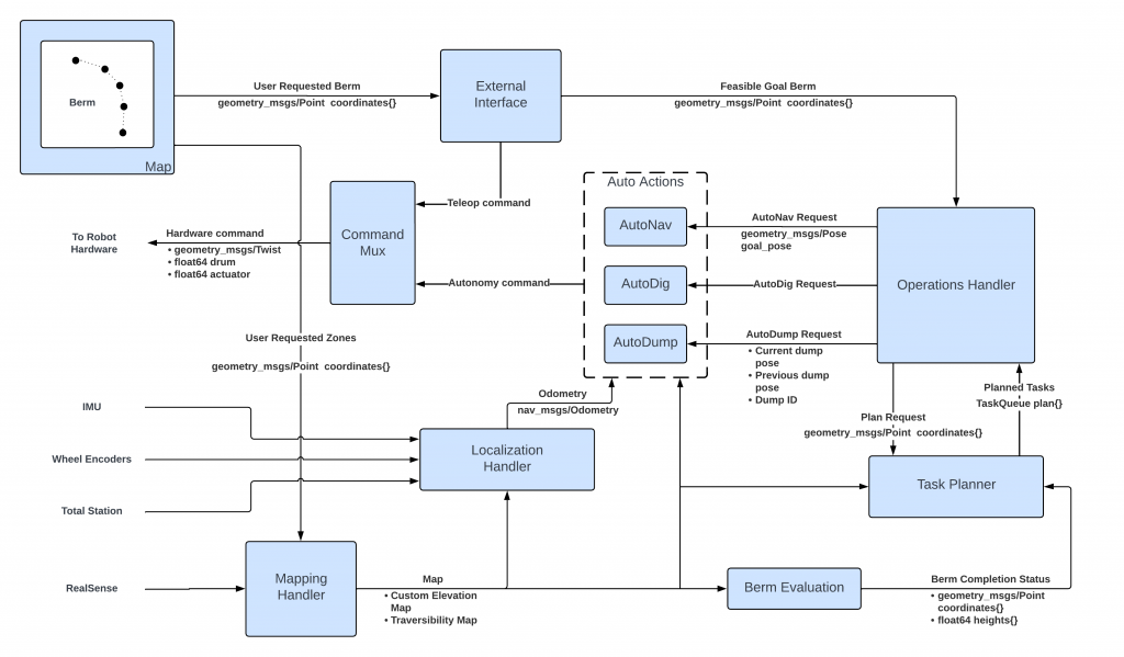
The first is the autonomy container, which consists of all software packages responsible for the autonomous operation of the system. The autonomy software elements along with their interfaces are visualized in the figure below. The pipeline begins with the user marking the desired berm configuration, restricted zones and excavation zones on the control station. These point coordinates are processed and then passed on to the rover. The ’External Interface’ node, which is responsible for all communication with the operator, checks these desired berm coordinates for feasibility. This node also enforces security locks in case of communication loss. The feasible berm coordinates are then provided to the ’Operations Handler’ node to start autonomous construction of the berm. A plan is fetched from the ’Task Planner’ node, which is used by the operations handler to respectively call the AutoDig, AutoNav and AutoDump actions. The ’Command Mux’ node selects which command will be used to drive the system at any given moment. This is provided for efficient switching between teleoperation commands from the user and the autonomous commands from the system itself. The ’Mapping Handler’ and the ’Localization Handler’ nodes keep the terrain map updated while also keeping track of the system’s pose within that map. The ’Berm Evaluation’ node gives crucial feedback on the progress of the construction to the task planner to dynamically re-plan if required.
The second container is the hardware-interface container, which contains all software packages required to control and communicate with the lower-level hardware. These include the package for controlling the Husky mobility base and processing data from the IMU, RGBD Camera, and tool encoders. This container communicates with the Arduino Mega microcontroller that is employed to control the tool subsystem.
Localization
An accurate pose estimate of the rover’s position with respect to the berm it is building is required for autonomous operation. The localization subsystem makes use of the total station, wheel encoders, IMU, and tool encoders to estimate the system’s pose within the work site. As the position feedback from the total station is discontinuous, two different odometry streams are generated. Local odometry is generated by fusing the data from the wheel encoder and the IMU using an Extended Kalman Filter. This fused data is guaranteed to be continuous for a short period of time in the local frame. Odometry for the global frame is generated by using another Extended Kalman Filter that fuses the data from all the sensors to produce a highly accurate pose estimate in the global map frame. As the total station provides extremely accurate but discontinuous measurements, the covariance and the system process matrices are tuned such that the position estimate converges rapidly to the estimate from the total station. This ensures the system achieves reliable localization. We conducted loop closure tests and measured the loop closure accuracy of our localization subsystem to be under 2 cm, hence demonstrating the capability of this subsystem.
Task Planning
The task planning subsystem plays a vital role in optimizing the construction of the berm for efficiency by devising a feasible high-level task plan. Maneuvering through a 3D environment while manipulating terrain offers numerous possibilities for constructing a berm. For instance, in the scenario of a straight berm, the initial layer might follow a straight line, and subsequent layers could be deposited at the same locations, in between sections, or randomly distributed. Additionally, exploring multiple dumping positions within a single excavation cycle adds to the complexity. Planning an optimal sequence of dump operations in this expansive and continuous space poses a computationally challenging task. To simplify the problem, the task planner operates under the following assumptions:
Assumption 1: The desired berm configuration can be segmented in the X-Y dimension, completing the entire berm by building each section.
Assumption 2: The angular change between any two consecutive berm sections will always be less than or equal to 10 degrees.
Assumption 3: Each operation cycle comprises a sequence of excavation, transportation, and deposition, all occurring only once.
In the process of experimentation, the length of each berm section, accommodating angular changes from 0 to 10 degrees, was determined to be approximately 45 cms. Furthermore, the number of dumps required in each section remains constant since the desired height for the entire berm is uniform.
Streamlining the problem to one dimension, the task planner processes feasible excavation sections and computes an optimal sequence for visiting and depositing material in the berm sections. At a high level, this problem mirrors a traveling salesman problem with state-dependent movement costs. Each construction of a berm segment introduces an obstacle to the costmap, altering the cost of visiting all remaining berm segments. Since our transition costs are solely a function of the state, we frame the problem as a bi-level optimization scenario. The top-level planner engages in a graph-based search to uncover a feasible min-cost solution. Simultaneously, at the lower level, a hybrid A* planner calculates the edge cost. Our approach also uses a TSP-based heuristic, which solves a relaxed problem to accelerate the top-level search. The low-level graph search problem involves the navigation of the robot from the excavation zone to the desired berm section. For computing the TSP-based heuristic, our approach leverages the Google OR-Tools TSP Solver, employing an octile distance matrix between each state. The octile distance, not factoring in collisions, provides an underestimation of the material transport cost between the excavation and berm sections. Additionally, as we don’t need to return to the start node, in contrast to the general Traveling Salesman Problem, we set the cost to reach the start state as zero from all other states. This effectively neutralizes the impact of reaching the starting node at the end. In the distance matrix, we assign a zero cost to travel to the same node or go to any excavation zone. When traveling from the start excavation zone to a segment, we choose the minimum octal distance to reach any dump pose for that segment. Finally, for traveling between segments through an excavation zone, we again select the minimum across all potential transitions to consistently underestimate the cost.
AutoDig
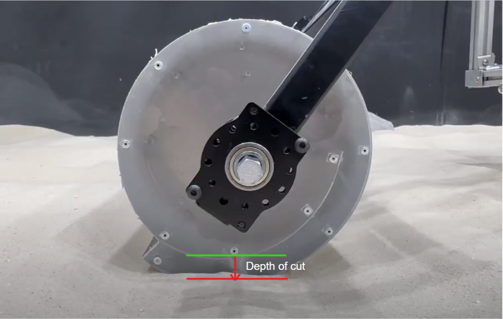
To dig material from the ground while maintaining low ground reaction forces, the tool needs to be lowered to its desired depth of cut and rotated while the robot is moved forward. The height of the tool needs to be adjusted dynamically throughout this maneuver to account for uneven terrain and maintain excavation efficiency.
We use two intuitive observations to design a controller for this purpose. The first observation is that if there is more material present inside the drum, it consumes more power and, hence, more current to rotate it. Secondly, if the tool excavates too deep, it will also consume more power (and therefore current) to excavate. Therefore, tool current feedback is incorporated and used with a cascaded PID controller to command the tool’s depth of cut. This helps track a desired tool current profile.
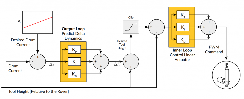
The outer-loop of this controller predicts the delta dynamics of the system: given an error in the currents, it predicts the change in height required in order to stabilize the current errors. This differential is then added to the current tool height estimate, which is used by the inner-loop PID to command the linear actuator. To reduce the initial overshoot, which could occur if the start tool height is very far from the desired tool height for excavation, absolute ground height measurements from the point cloud were used. This absolute height helped initialize the tool’s excavation height at a suitable position. Data from manual excavation operations was used to calibrate the profile of the target current trajectory and tune the outer-loop proportional gain. This methodology helped achieve robust operation across a variety of uneven terrains.
AutoNav
The Autonomous Navigation (AutoNav) subsystem facilitates the robot’s movement to efficiently transport excavated material from the excavation region to the designated berm section. The primary challenge involves navigating through a high-resistance and deformable sandy terrain. Although the Clearpath Husky is a differential drive robot that can take point turns, i.e., rotate in place, we avoid this to prevent creating grooves in the terrain, rendering it untraversable. Therefore, the AutoNav subsystem generates a smooth path, incorporating a minimum turning radius constraint of 2.5 meters.
The AutoNav leverages the ROS 2 Nav2 Smac Hybrid A* path planner to generate a smooth trajectory, utilizing Reeds-Shepp motion primitives. This choice not only ensures a smooth trajectory but also introduces the valuable capability of reverse movement, a feature absent in Dubin’s path. To track the generated path with precision, AutoNav employs the Regulated Pure Pursuit controller from the Nav2 package.
However, the controllers in the Nav2 package were initially designed for flat terrains and may not be optimized for sandy landscapes. Given the deformable nature of the terrain and potential localization errors, achieving perfect tracking, especially during turns, becomes challenging. In response to these real-world complexities, AutoNav takes a proactive approach by dynamically generating a new path plan every 5 seconds. This adaptive strategy allows the controller to automatically commence tracking the freshly generated path, mitigating issues associated with deformable terrains.
AutoDump
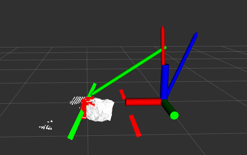
The primary objective of the AutoDump subsystem is to correct the navigation and localization errors and deposit material in the right position in order to minimize construction errors. The first step in this process is to detect the previously built berm in the region near the present dump location. A median based clustering method was implemented to segment the berm in the point cloud, followed by RANSAC to fit the peak line of the visible berm. After detecting the peak line, the segment ID of the detection in the point cloud was identified by finding the berm segment that has the centroid closest to the detected peakline. Using this information, the target deposition point is recalculated using the input berm geometry. This point is then used to calculate the errors in the distance x, yaw angle phi, and tool height. A complementary filter is added to the error estimates to ensure robustness single frame detection failures.
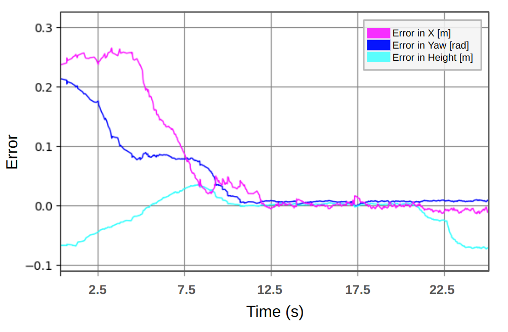
Three parallel PIDs are used to mitigate the errors generated by visual servoing. The rover is moved to the correct position and tool height for dumping material. Finally, the rover deposits material at this position by rotating the drum until it is empty and raises the tool back to its highest point, marking the end of one AutoDump cycle.
Pointcloud Processing
The decimation filter provided by RealSense ROS libraries was used to first sub-sample the point cloud. Given the pointcloud stream in the camera frame, the pointcloud must be processed to the robot base link frame and filtered to be useful for downstream perception algorithms.
To achieve this, we first get the static transform from the camera frame to the robot base link frame and apply eigen transformations in the fixed frame to the pointcloud data. Next, we subscribe to the tool height and appropriately crop out the points corresponding to the tool. This is important since the visible tool would hamper performance in the downstream perception tasks, none of which require the tool points. Finally, we perform noise removal by outlier detection and publish the resultant pointcloud in the robot base link frame.
Mapping
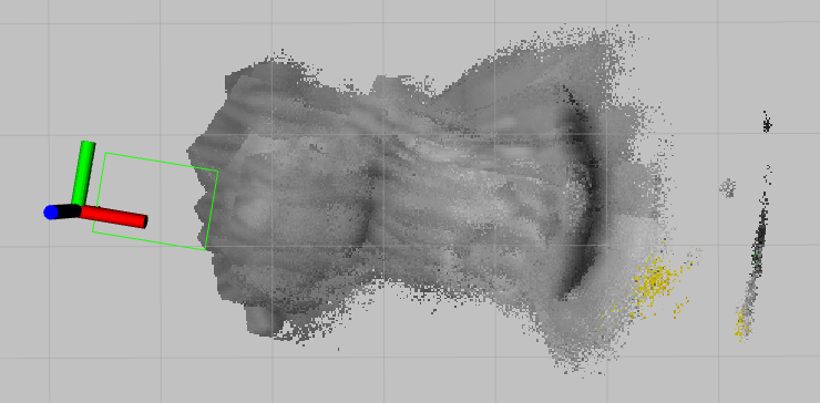
The mapping subsystem uses various inputs like the transformed pointcloud in the robot base link frame, the robot’s pose from localization, user-defined berm locations, and predefined restricted zone coordinates. Its goal is to generate a global elevation map, track berm progress, and create a traversability costmap.
The map frame is centered at the moonyard’s center, aligned with Total Station axes, and has a resolution of 1.5cm, resulting in an 800×800 grid where each cell holds the average elevation in that area. To build the elevation map, the processed pointcloud is transformed to fit the map frame, and then divided into map resolution bins. Each cell in the map is treated as a Bayes filter unit to accommodate Total Station prism and camera sensor mast vibrations.
For the AutoNav subsystem’s traversability costmap, we create another grid within the map frame, initializing all cells as 0 (denoting traversable terrain). The process involves setting the moonyard walls to a cost of 100 to indicate them as obstacles. Then, areas defined by the restricted zones receive a cost of 100 by identifying intersecting cells within the polygon specified by the restricted zone coordinates. Finally, the desired berm regions are marked as cost 100 to ensure the rover avoids disrupting its own construction.
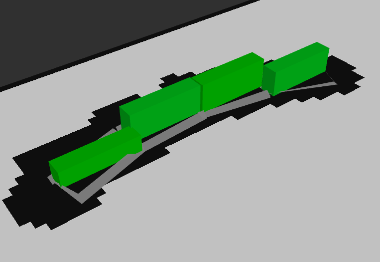
Berm Evaluation
To plan and re-plan autonomous construction operations, accurate measurement of the progress is required. This will allow for the planning of the subsequent excavation and build-poses. The berm evaluation unit subscribes to the map and interfaces with user inputs for desired berm configuration and pre-defined restricted zones.
To evaluate the berm, the height, length, volume and positional error are calculated. Given the desired berm points, the berm is segmented into sections of length equal to the drum length. For each such section in the global elevation map, the 95th percentile height is reported as the height in each section, and the average of berm section heights is reported as the height of the berm. To calculate the length of the berm, the berm region is binned and peakpoints are selected as maxima in each column perpendicular to the berm section. The ground elevation is estimated by the average elevation map value in the region between 40 to 50cms of the neighborhood of the berm region. The number of columns with minimum 70% of the berm section height are counted as peakpoints and its product with the hypotenuse of patch size is reported as the berm height.
The volume of the berm is estimated by summing up the elevations in 30cm neighborhood of the desired berm peakline and marking it with the timestamp. The error in construction is computed by taking root mean square (RMSE) error of the current berm peakline obtained through binning to the desired peakline.
External Infrastructure
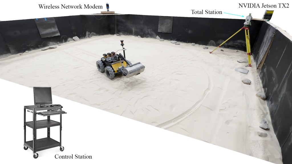
The external infrastructure is the combination of elements that are not onboard the system but are necessary for operation. It includes the control station, joystick for teleoperation, interfaces for wireless communication, and total station for localization. It also includes evaluation tools such as a FARO laser scanner or an external RGBD camera to evaluate the final worksite configuration. The wireless network over which the robot, control station, and the total station communicate has been visualized in the figure.