Software CodeBase
Our codebase can be found at our GitHub workspace (Running instructions can be found in respective ReadMes):
- rsun_goal – Utils and Launch files for physical/simulation UAS bring-up – branch: fuel-cer-hw
- rsun_fire_localization – Scripts for running our new perception pipeline – branch: main
- rsun_goal_planner – Personal copy of open source project with relavant mod – branch: p2p_hw
- fast_exploration_planner – Personal copy of open source exploration mod – branch: fuel_cer_hw
- rsun_autonomy_simple – branch: fuel_cer_hw
- rsun_gcs_streaming – branch: hw_mods
- rsun_drivers
Spring and Fall Semester Implementation
The following description about our subsystem implementation is distributed into two broad time periods: the Spring semester and the Fall semester. The fire localization and the state estimation subsystems were of major focus in the spring semester, however in the interest of a successful demonstration and realism to our use case, we took decision in the fall semester which extensively changed our subsystem design as compared to the spring semester including designing a new drone. To explain this aptly, we first describe the implementation summary of the fall semester, referring to the spring semester implementation details along the way. The spring semester work would be displayed below the fall semester work.
Fall Semester
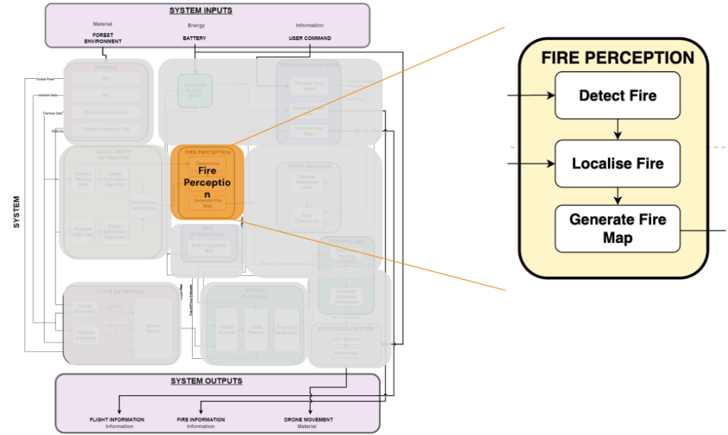
[Revamped] Fire Perception
Fire Localization in Phoenix: In our previous aerial system, Phoenix, the fire localization module processed thermal images to determine fire hotspot coordinates for mapping. Two methods were explored: a learning-based approach developed by AirLab and a classical method developed by our team.
The deployed method relied on classical stereo matching of synchronized thermal feeds, rectified using OpenCV’s stereoRectify to correct distortions. Temperature-based masks were generated to segment hotspots, and ORB features were then detected and matched between the left and right frames. The matches were refined using epipolar constraints to estimate depth and compute 3D coordinates in the world frame.
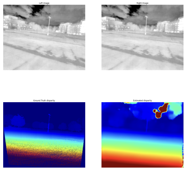
Alternative approaches included generating disparity maps with StereoSGBM and using Fast-ACVNet for learning-based depth estimation. These methods showed promise but faced challenges such as information loss during image conversion and poor performance due to distribution mismatches.
While Phoenix Pro employs a different fire localization system, these efforts informed our understanding of thermal-based perception.
In the Phoenix Pro system, the fire perception module was designed to localize and map fire hotspots more accurately compared to the previous approach used in Phoenix. The previous system relied on a thermal stereo-based design, which exhibited a localization error of approximately 2 meters within a range of 5 meters. This approach faced several challenges, including the requirement for a large baseline between thermal cameras and the difficulty of performing precise extrinsic calibration between them. These factors contributed to inaccuracies in fire localization, limiting the effectiveness of the system for real-world applications.
Fusing RGBD and Thermal
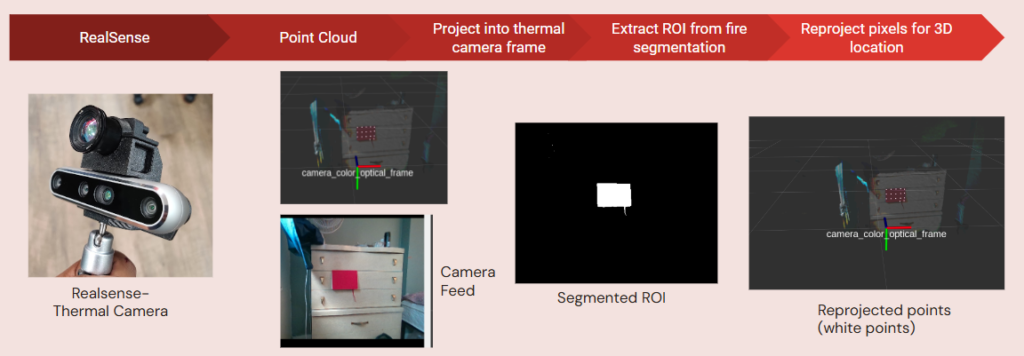
To overcome these challenges and improve localization accuracy, we adopted a new approach in Phoenix Pro that leveraged the RealSense point cloud, effectively bypassing the need for thermal stereo. The RealSense camera provided dense RGB-D data, enabling us to obtain accurate depth measurements without the need for large baseline configurations or complex thermal camera calibration. By integrating thermal information with the RealSense point cloud, we could project fire hotspots detected in the thermal images into 3D space with higher precision. This method significantly enhanced the accuracy, localizing fires now up to 50 cm error for a 6 m range.
The overall flow of information from the sensors (FLIR Boson + RealSense D456) to the fire localization and mapping is depicted in the figure below. We receive data from FLIR Boson at 30 fps, and point cloud from RS D456 at 30 fps. We first downsample the point cloud with a leaf size of 0.1 m, and clip the range to 8 m. This reduces the computational load and filters out bad points in the point cloud. With this configuration, we are able to achieve localization at 30 fps, i.e., in real time.
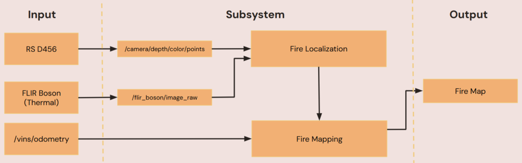
We do a binary segmentation of fire hotspots, transform the point cloud into FLIR Boson’s optical frame using RS-Thermal extrinsics, and then project the points onto the FLIR’s frame using the intrinsic parameters of the FLIR. We reproject only the pixels corresponding to the hotspots using the mask, and then publish the centroid of the reprojected points. For tackling multiple hotspots, we cluster the segments in the binary mask generated from the thermal image using OpenCV’s connected_components. Clustering in 2D image space rather than 3D space reduces the computational overload significantly and enables real-time operation. This is depicted in the following figure.
Note that the range of the point cloud affects the fire perception capability during exploration. This parameter should be set based on the depth range assigned in the exploration. If the drone performs less exploration, then it is advised to set a longer range. However, this would affect localization accuracy due to poor points from the RS D456.
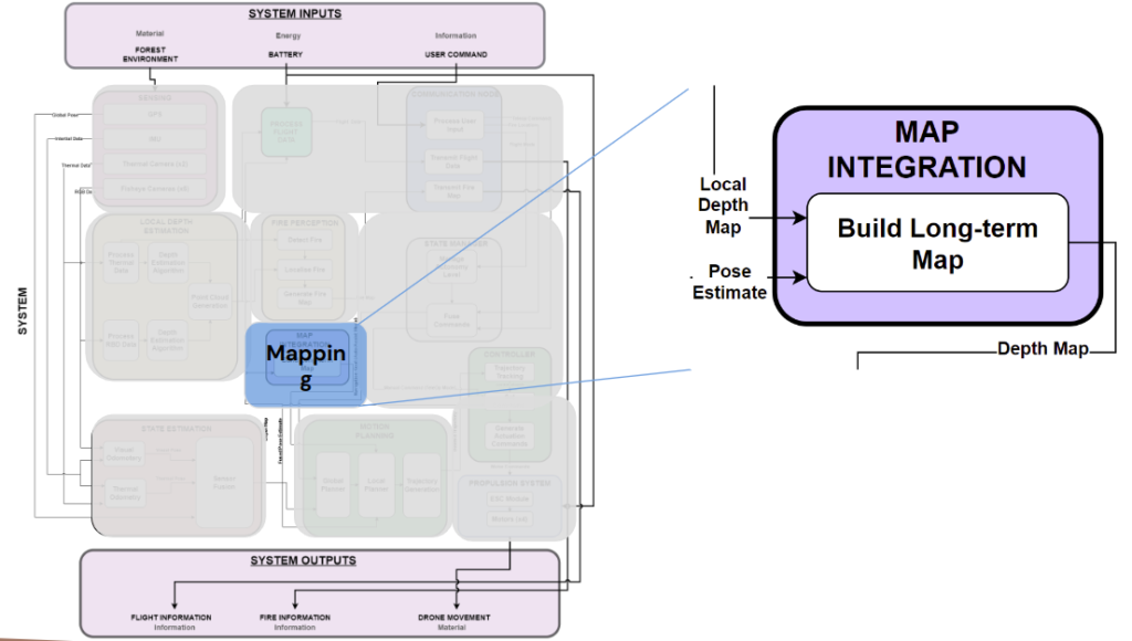
Global Fire Mapping
Similar to the Spring semester, the global fire mapping subsystem handles the temporal side of the fire perception subsystem. The fire perception module provides raw measurements of hotspot locations relative to the world frame. When the fire perception subsystem publishes a new set of measurements, this mapping subsystem is executed as shown in the flowchart above.
Note: Unlike the Spring where we had a dedicated filtering module, the introduction of RGBD-Thermal fusion significantly enhances the quality of our raw measurements. Specifically, moving away from the triangulation approach, there are now no false positives behind the camera.
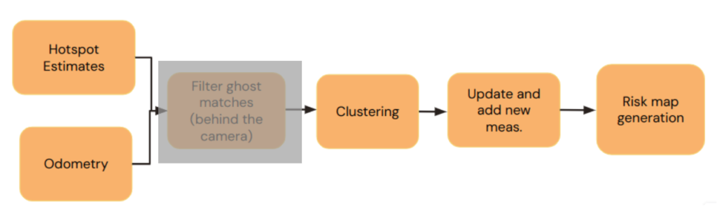
Adding New Hotspot: We then perform nearest neighbor clustering for each hotspot to determine whether it is a measurement for a new or existing one. A new hotspot is created if it exceeds distances from all previously seen hotspots.
Updating Existing Hotspot: If we instead find any measurement corresponding to an existing hotspot, we add it to the existing nearest-neighbor map, and use a mean search to find the updated position of its parent hotspot.
[Revamped] State Estimation
In line with our non-functional requirement MNF4, which mandates the use of passive sensing modalities, and considering the GPS-denied environment in which our system operates, we developed the state-estimation module to use two NIR cameras and an IMU sensor as inputs to estimate visual odometry.
VINS Fusion
We choose to use off-the-shelf VINS Fusion which is an optimization-based multi-sensor state estimation package due to its wide adoption in the robotics community and its recognition for robustness.
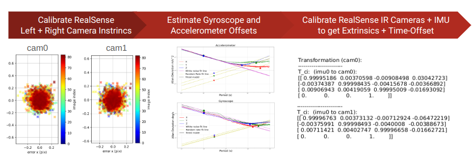
The key prerequisite for using the package with an IMU and cameras is to provide accurate IMU-to-camera extrinsic, camera intrinsics, IMU gyroscope and accelerometer biases (noise), and the time offset between the IMU and camera topics. The figure below shows the calibration pipeline developed to accomplish these tasks. Initially, Kalibr calibration package is used to obtain the camera intrinsics for the RealSense left and right NIR cameras using a checkerboard pattern. The imu_variance_ros package was then used to estimate the IMU biases, which were subsequently used by Kalibr to perform the calibration and obtain the IMU-to-camera extrinsic (for both cameras) and time offset.
Overall Pipeline
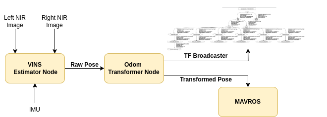
The flow of our state estimation module is illustrated below. The VINS node uses an IMU sensor and two NIR (Near-Infrared) images from the left and right cameras of the RealSense D456 to estimate the odometry. This data is then processed by the Transformer node, which publishes the odometry at a fixed rate of 25Hz, transformed with respect to the UAV platform’s base-link frame. Additionally, this node is also responsible for broadcasting the transforms between the map, IMU, odometry, base-link, and thermal camera to the RealSense depth frame.
Note: In the Fall, we decided not to use Multi-Spectral Odometry (MSO), previously used in our Spring Demonstration. The decision was based on its limited documentation, tight integration within a Docker environment on ARM-based hardware (ORIN on ORDv1), incomplete code commits, and the departure of its key developer from Airlab, making it difficult to integrate into the new platform (Phoenix Pro).
State Manager
FSM States
To keep track of the overall state of the system, we have some central states which are the minimum essential for aerial systems. These are:
- GROUNDED: System on the ground in unarmed state.
- TAKEOFF: System takes off and reaches desired height.
- HOVER System in offboard mode. holding positions, awaiting interface state change.
- ACTIVE_P2P: Active in P2P navigation mode
- ACTIVE_EXP: Active in exploration mode
- LANDING: System landing (in case of mission end or failure)
- END: Mission end, disarm, no further transitions.
- FAILURE: System level failures – asynchronous
These states help us implement logic for the entire mission. Inside the Active P2P and EXP states we have further internal states inside the P2P and Exploration modules. These internal states handle the inner logic and help the central manager understand what’s going on inside the individual packages. These internal states are:
- PRE_INIT : Pre-initialization phase to allow checking for inputs to either planner or exploration.
- INIT_READY: Above checks pass, system ready to receive goal
- ACTIVE: System is executing task ( p2p navigation or exploring an area )
- DONE: Successful completion of task
- FAILURE: Can happen at any step during the execution of task.
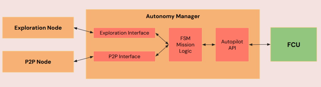
Central Manager
With the information about the system and the individual packages from above defined states, we have our mission logic inside the central manager. This handles the following tasks sequentially:
- Arming the drone and takeoff commands using MAVROS API
- Switch to OFFBOARD mode and checks
- Once in OFFBOARD, and if overall system status in HOVER, switch to ACTIVE_P2P
- Once a goal is given, P2P goes to ACTIVE
- If there is no Failure, and P2P is done and system inside exploration region, switch to ACTIVE_EXP
- Once exploration is done, and there is no failure, go to LANDING.
The rough plan explained above has checks in between to ensure correct state transitions. Using these state transitions, when exploration is done, we can switch back to ACTIVE_P2P mode and give the goal as home base however this was not demoed at FVD due to lack of testing time, but this was tested successfully in simulation. These state transitions were logged in real time so that the operator knows the current state of the system. This was especially helpful to us during testing.
Mapping + Motion Planning + Trajectory Generation
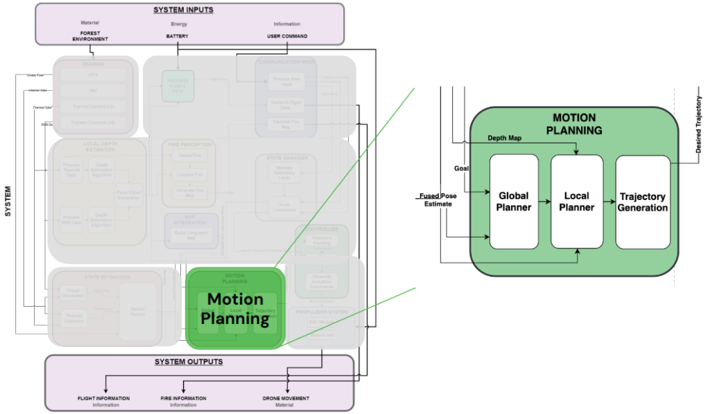
The above three mentioned modules are incorporated by the open source packages that we use for performing two tasks: Point-to-Point Navigation, and Exploration. The former allows the user (or firefighter) to give an initial goal to the drone inside the “dangerous area”. The P2P module generates a safe trajectory around the obstacles, and minimizes the path length. Once the drone enters the dangerous area and reaches it’s rough goal, it uses the Exploration module to survey the entire area for hotspots while avoiding obstacles. These modules are explained in depth below along with our modifications to port them into our system
Point-to-Point Navigation
To demonstrate a realistic enactment of our use case, we wanted to give a rough goal to the drone inside a “dangerous area” where we want the drone to explore, map the environment for hotspots and return this map. To get the drone inside the dangerous area, we looked for an open source implementation capable of autonomous path generation and obstacle avoidance given a goal.
We decided to go with CERLab’s work for navigating in presence of static and dynamic obstacles (we were only interested in static obstacles). This package was easy to setup and run, and our plan was to detach the controller from this package, and use the trajectory generation output and feed the waypoints into our autonomy manager which can then further handle sending these waypoints to PX4’s inbuilt controller.
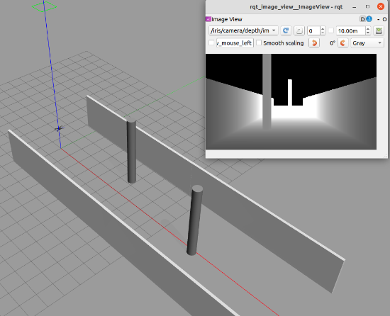
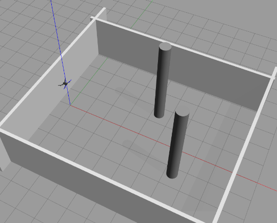
After initial tests, a simulation world similar to our testing site at NREC’s Drone Cage was setup to test this package with a model of the drone (IRIS) with a depth camera plugin, and our autonomy manager.
Exploration
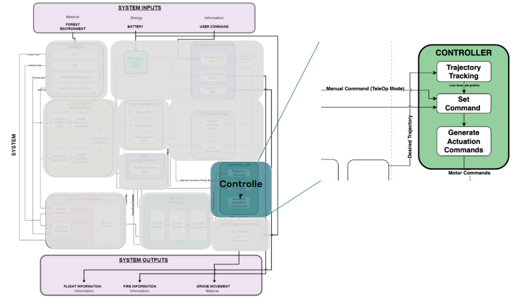
Controller
Autopilot API

This is the underlying Python library used Autonomy Manager for interacting with the FCU. This library was developed from scratch. MavrosAPI as the name suggests acts as the Python wrapper around the ROS interface utilities provided by MAVROS. MAVROS in turn acts as the ROS wrapper for MAVLink communications, enabling control over the PX4 Autopilot functions via MAVLink running over serial.
Some utilities provided by the API library:
- Autopilot Failure Monitor
- Autopilot Arm/Disarm
- PX4 Parameter Validation/Overrides
- Autopilot Flight Mode Configuration
- Auto-Takeoff
- Waypoint Navigation
- Trajectory Tracking
- Auto Landing
Spring Semester
Fire Perception
Implementation [Exploration Phase]
- Fire Segmentation: The fire segmentation pipeline processes raw radiometric readings by both left and right cameras, and converts them into easily readable temperature values, typically measured in Celsius. Following this conversion, a binary segmentation pipeline is used to isolate the fire hotspot region by masking out all pixels below a predetermined threshold value, effectively highlighting the area of interest. Additionally, another pipeline is available to conduct slab-wise segmentation of the temperature map, allowing for a more detailed analysis.
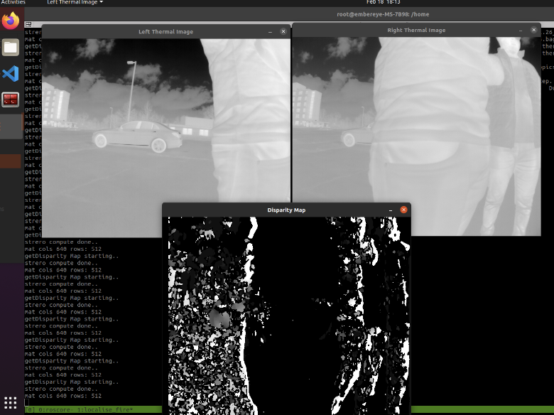
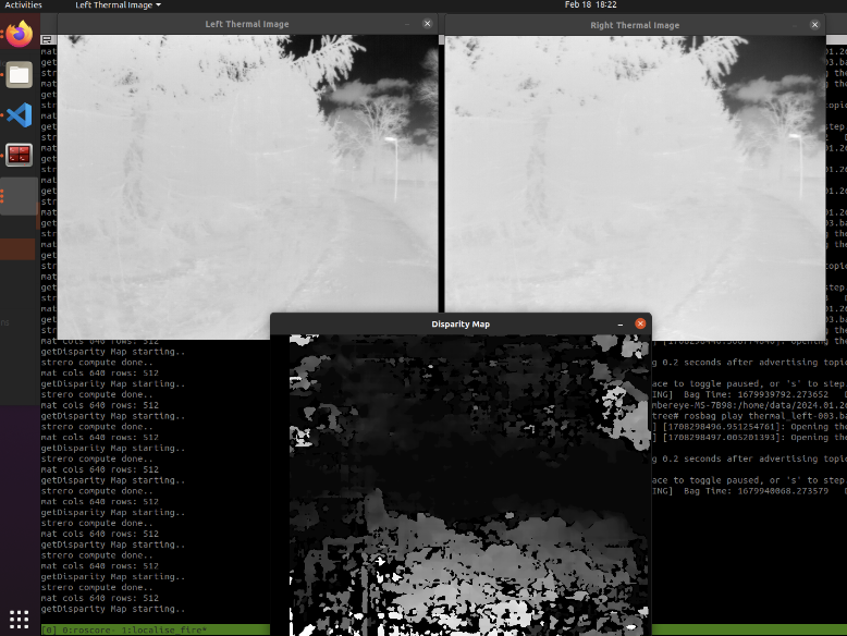
- Fire Localization: In the development of the fire localization system, several methods were explored but encountered various challenges. The first approach utilized the OpenCV StereoSGBM module to generate disparity maps from thermal stereo images. This method faced issues with accuracy due to the necessary conversion of 16-bit images to 8-bit, resulting in significant information loss (image smoothing and noisy disparity maps). An enhancement was attempted by performing image processing of the rectified thermal images; however, this improvement yielded minimal enhancement in the feature-matching process. Lastly, a learning-based method using a Fast-ACVnet architecture was trialled, which showed promising results with disparity maps achieving a performance of 13 frames per second. Despite some artefacts, the depth estimation near the ground was reliable, suggesting potential for practical application in fire mapping. Although the results from the learned model were good, this approach can not be used for our application since the space heaters that were used for simulating fire were out of the distribution of the model. Hence the learning-based model produced poor results on our test site. The results for these approaches are attached in the figures attached below.
- Fire Mapping: The fire mapping pipeline takes into input the three major upstream subsystems, ie., fire segmentation, fire localization (thermal depth estimation), and VIO, and fuses them to give the locations of the hotspots in the world frame. This is done by first performing clustering of the hotspots in the image plane (using the segmented mask), then projecting these hotspots in the camera frame (3D) using the depth image, and ultimately in the world frame (using VIO).
Implementation [Deployment Phase]
Under this section we briefly explain the final working pipeline that we went ahead with for our SVD. The high-level steps to calculate the coordinate of the hotspots and append them in a map were as follows
- The feed from left and right thermal camera image are first rectified using cv2’s stereoRectification funciton using the camera’s distortion coefficients.
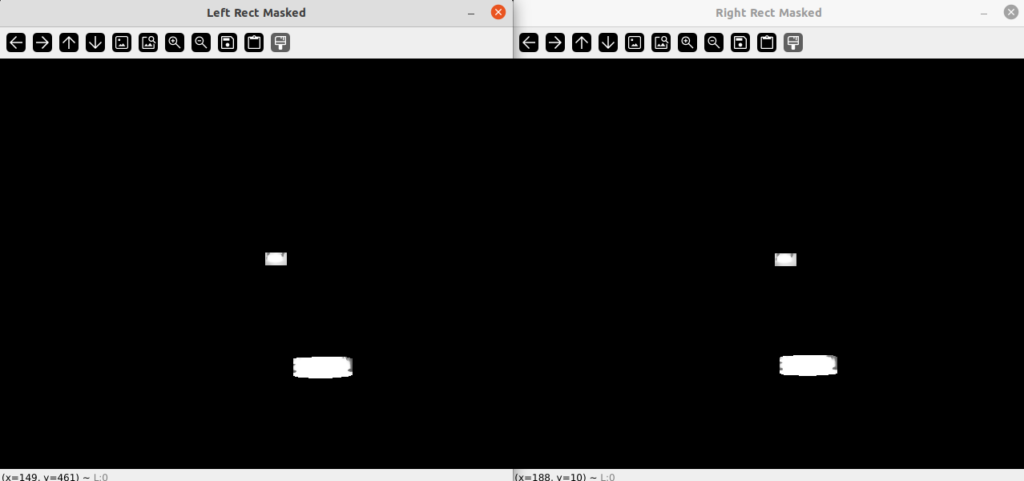
- The rectified image is then converted to a temperature based binary image. This is explained in the segmentation technique above.
- The mask generated from the temperature mapping is used on the rectified feeds to isolate out the hotspots and their surrounding area.
- On these areas, we detect ORB features and compute key-points and descriptors for the same.
- These features are then matched using a Brute-Force matcher and then filtered out using epipolar constraint.
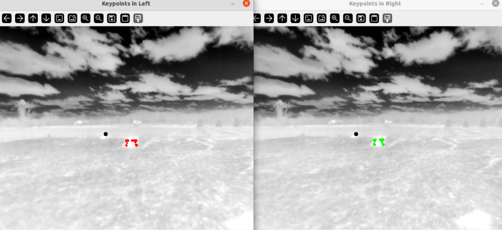
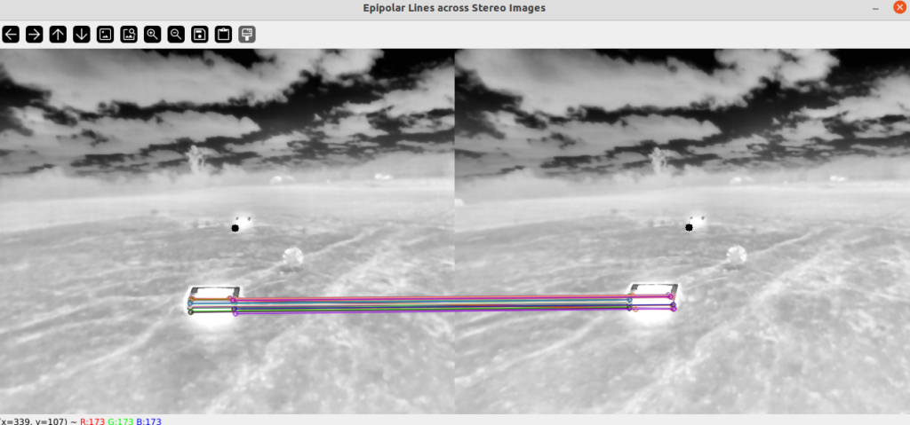
- Only those matched features are selected, which are closer to the epipolar line of their corresponding match in the other frame.
- Using these good matches, we calculate disparity, and eventually depth using the baseline information.
- Using proper transformations now we can calculate the 3D coordinate of the hotspot in world frame.
Fire Localization (Global Mapping)

Our global mapping subsystem handles the temporal side of the fire perception subsystem. The fire perception module provides raw measurements of hotspot locations relative to the world frame. When the fire perception subsystem publishes a new set of measurements, this mapping subsystem is executed as shown in the flowchart above.
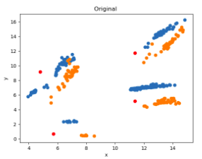
Filtering: Once we receive a hotspot measurement, we first need to filter out the good readings, because most readings are quite noisy. The following are the 2 main filters we employ. Figure below shows the measurements from 2 successful flights (L) and the measurements after filtering (R). The red spots show the ground truth hotspot locations.
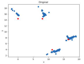
Adding New Hotspot: We then perform nearest neighbor clustering for each hotspot to determine whether it is a measurement for a new or existing one. A new hotspot is created if it exceeds distances from all previously seen hotspots.
Updating Existing Hotspot: If we instead find any measurement corresponding to an existing hotspot, we add it to the existing nearest-neighbor map, and use a mean search to find the updated position of its parent hotspot.
Implementation
Multi-Spectral Odometry: is a package we used from Airlab which uses a set of cameras (RGB, Thermal or a combination). The algorithm detects features in the image captured by the cameras, tracks the motion of the features as the robot platform moves and estimates the state using this information. A brief description can be seen in the following slide images:
Frame Transformations:
The MSO odometry data is estimated concerning the primary camera optical frame. For use of this data for autonomous flight with PX4, the estimates need to be transformed to a body-fixed FLU frame (centred at the IMU of the FCU). We incorporated the camera-IMU extrinsic data from Kalibr to perform this transformation.
Indoor hand-held Test: To test the drift and RMSE of the multi-spectral odometry and the IMU propagated odometry, we perform some indoor tests by dragging the Phoenix on a cart around the lab to make a path of more than 100 meters.
The 100 meter path shows a final drift of less than 1% ( of 0.912m with path length 116.562m ). Note this is using the upward looking camera in the left-front. In the field we would be using the downward facing camera in the front with appropriate mask to hide the landing gear and the sky that shows up around the edge of the fisheye feed due it’s more than 180 degree fov.
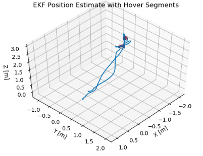
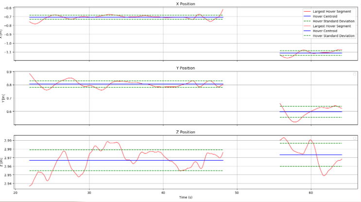
Outdoor Flight Test (Hover): (Location: Nardo)
We perform a hover test with the following criteria:
- No pilot input is given to the drone
- Less than 0.1 meter drift during the hover period
- Hover period should be of more than 5 seconds
Video Link to hover flight footage at Nardo: https://drive.google.com/file/d/1F5KQ4VgDD9Ojskx4JA-1q7zFz8-oaJRF/view?usp=drive_link
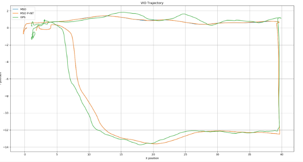
Outdoor Flight Test (Loop): (Location: Nardo)
Loop flight footage: https://drive.google.com/file/d/115YwKfgc7a4GouLOdBDppV8XkNJJ0_i0/view?usp=drive_link
The drone was flown in a loop to evaluate the MSO drift metric in the field when compared to the GPS data. The resulting drift was of around 1.6m for a path length of 105.47m. This satisfies the performance metric that was set ( < 4% drift for a path length of 100m ).
Failsafe Policy for MSO:
As VIO by nature is unreliable in HDR and feature-sparse settings, we always need a failure detection logic to trigger appropriate failover. Some systems use the estimated confidence/covariance to make this transition. But as our VIO system does not offer such quality metrics, we rely on simple but effective data sanity checks incorporating raw IMU data and kino-dynamic limits of the system.
Having such a failsafe helps us prevent catastrophic loss of the system and/or lives.