
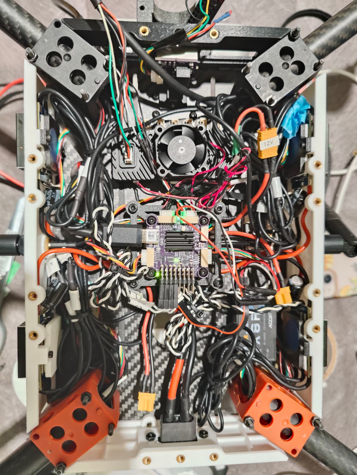
Hardware
Low-Level Sensor integration
Thermal Cameras: The drone uses 2 FLIR Boson cameras giving us 640×512 resolution. We wrote our own custom driver using V4L2 to allow for quick processing and efficient memory management. The driver also allows the thermal camera to be set to disabled, master, or slave mode and this changes the timing characteristics of the cameras. We have also developed a thermal preprocessing method that takes into account thermal-sensor noise adjustment using FFC, gain correction, histogram equalization, and noise estimation.
RealSense 465: This is to measure ground truth and provide some depth estimation when flying outdoors or in environment where visual features can be leveraged. The RealSense has 2 imagers, 1 color sensor and 1 IR projector along with an internal IMU.
IMU: The drone relies on 2 Inertial Measurement Units – Epson G365 external IMU and one that is included with the RealSense 465. The team has worked towards improving the Epson IMU driver code as by-product of testing and debugging issues with it.
Mechanical Design
The integrated hardware for the drone includes:
- Nvidia AGX Orin for onboard compute,
- 2 Flir Boson cameras for thermal vision,
- Intel Realsense D456 for RGBD ground truth data collection,
- LiPo battery for power,
- Pixracer Pro for flight controller,
- Ainstein US-D1 radar for altitude sensing,
- Epson G365 inertial measurement unit, and
- Frsky X8R radio receiver for manual teleoperation signal
All built on a Hexsoon EDU-650 airframe.

All components were designed for modularity, ease of manufacturing via 3D printing, and ease of assembly. The three main subassemblies in the mechanical design are the thermal camera subassembly, the Orin subassembly, and the battery subassembly.
In the thermal camera subassembly, each thermal camera is attached to the airframe and secured in all degrees of freedom by three parts: the camera lid, the mount arm, and the mount lid. The camera lid is fastened to the camera itself and the mount arm, the mount arm is further fastened to the mount lid and the front plate of the airframe, and the mount lid is then fastened to the top plate of the airframe. This mounting strategy was designed to ensuring Single Fault Tolerance, ie. the subassembly will remain securely attached even if any one set of fasteners become loose. Furthermore, the camera placement and consequently length and shape of the mount arms were set to ensure no obstruction to the camera field of view from the airframe. Additionally, custom crash protection bumpers were designed to take the brunt of any impact forces while also staying out of the camera field of view.

The Orin subassembly consists of a cap and foot fully covering the Orin from the top and bottom. Fasteners go from the cap, through mounting holes on the Orin, to threaded inserts in the foot, securing the Orin within the enclosure while the enclosure design leaves sufficient clearance for the internals. The foot of the enclosure is secured to the drone airframe via a mounting board or it can be removed as a standalone unit, allowing the Orin’s enclosure to be separated from the airframe as an independent subassembly for parallel development.
The battery is held up by three concentric rings and held in place at the ends by two interference fit bookends. The elastic deformation forces secure the battery position with flexibility for battery shape variations. The Ainstein radar is mounted to the bottom of the concentric rings via a mounting plate, since this is the best mounting location on the drone that allows the radar to be parallel to the ground plane and farthest from the landing gear or anything else that could get in the radar’s FOV. The radar is protected by its own custom crash protection bumpers similar to those designed for the thermal cameras.


Electrical
The drone now boasts 2 Flir Boson (Thermal) Cameras, an Intel RealSense (to collect ground truth), Epson IMU, an Ainstein Radar (Altimeter), Pixracer Pro (Flight Controller), Herelink airunit (wireless radio transmission), FrSky receiver, and an Nvidia AGX Orin as the host computer. The subsystem easily gets complicated and has to be meticulously designed with bandwidth and power consumption in mind. To provide the necessary power requirements, we have a power distribution board which provides us with 3 power lines – 24V, 12V, and 5V. The thermal cameras, realsense, and the IMU interface with the host computer allowing sophisticated algorithms to run onboard. The rest of the sensors and the host computer interface with the Flight controller allowing the higher levels of autonomy for the drone. Below is an example for how our sensors interface with the Nvidia Orin’s GPIO pins. We maintain copious documentation to keep the subsystem organized.

Flight Autonomy
The autonomy subsystem is the result of numerous complex subsystems working in synchronization with each other and the Flight Controller, enabling multiple levels of autonomy. Overall, through this subsystem we have delivered on one of the core requirements of firefighters – low cognitive load.
Before we list the capabilities of this system, it is imperative to emphasize that these capabilities were tested in both GPS denied environments and dense smoke. Below are the listed modes that the operator can interact with the drone in.
Level 1 – Stabilized Mode: Lowest level of autonomy where the drone stabilizes itself based on the IMU inputs. It is not robust to wind or external factors and the drone can drift easily.
Level 2 – Altitude Mode: Medium level of autonomy where the drone maintains its altitude and is robust to external factors that may change its altitude. Extremely stable for moving the drone around at a specific altitude.
Level 3 – Position Mode: High level of autonomy in which the drone holds its position and is robust to external factors like gusts of winds. Requires no operator inputs

Level 4 – Auto Land: Another high level of autonomy which allows the drone to land by itself without operator intervention. This mode has been particularly handy in situations where we lost communications with the drone. It safely lands itself saving us some crashes and rebuilds.


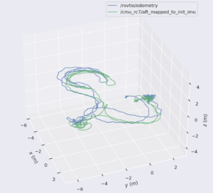
Odometry
The Odometry subsystem is responsible for predicting the drone’s change in pose over time. Throughout the semester, we explored and tuned a variety of algorithms for this purpose. Following advice from SLAM experts at Airlab, Shibo Zhao and Parv Maheshwari, we started by looking at Robust Thermal Visual Inertial Odometry (ROVTIO) and Uncertainty Aware Multi-Spectral Inertial Odometry (MSO) (authored at AirLab).
ROVTIO is an EKF-based odometry method that stores features for a short duration. Since it is EKF-based, it does not have a concept of loop closures and thus, does not benefit from revisiting old points. ROVTIO uses traditional feature detectors and is purely a classical approach. Since it is an EKF based approach, it does not have many parameters and thus can be tuned to work with any visual or inertial sensor relatively quickly.
MSO uses a factor graph-based approach which initializes variables and measurements and then optimizes to satisfy all constraints. It identifies features based on ThermalPoint, a feature detector that works on 16 bit thermal images. MSO is flexible enough that it can work with a vide variety of sensors but we are attempting to use it with one of the two mounted thermals or a dual-mono setup.
We initially benchmarked both these methods extensively on outdoor datasets (Caltech Aerial Dataset) and in large indoor spaces (SubT-MSO). Through these tests, we were able to glean a much more thorough understanding of both algorithms and their strengths.
However, when we tried implementing these algorithms on the Phoenix Pro system, the biggest challenge we faced with above methods were identifying the coordinate frames and how they are oriented. Although both algorithms accept IMU-thermal camera extrinsics, they have certain undocumented assumptions that makes it difficult to configure the hardware with the software effectively. For example, MSO accepts a gravity vector as a config parameter but the logic embedded in the code assumes gravity points in the negative z direction.
Following suggestions from our mentor at Airlab, we also began experimenting with Metrics-Aware Covariance for Learning-based Stereo Visual Odometry (MAC-VO), another odometry approach developed at Airlab based on estimating 2D covariances from a learning-based model and projecting these 2D covariances into 3D to determine optimal keypoints for feature tracking. We found significantly more success with MAC-VO and decided on this algorithm as the method of odometry for the spring semester.
To maximize MAC-VO’s performance as a visual odometry algorithm, we enhanced the testing scene with multiple thermal features such as humans, hand warmers, lights, and others, and made sure to traverse the environment slowly such that the algorithm could match as many keypoints possible across consecutive timeframes.
MAC-VO also supports swapping out the underlying modules that it uses for covariance estimation, keypoint selection, and pose graph optimization in a modular manner. Striving for a balance of performance and speed, the final configuration we went with, after much testing, was FlowFormer with covariance estimator for the frontend model, covariance aware keypoint selection, and two frame optimizer minimizing reprojection error.
Additionally to optimize speed, we parallelized running the frontend model on the Orin’s GPU and the optimizer on the CPU, as well as initializing MAC-VO’s underlying CUDA Graph Optimizer independently before initializing the Depth Estimation subsystem so that the CUDA optimizer would not capture any unnecessary inferences from the depth estimation model, FoundationStereo. The algorithm runs at about 1.6Hz independently onboard on the Orin AGX and 0.8Hz when run in conjunction with FoundationStereo.
Final System – ROVTIO
Throughout this semester, we worked on tuning and perfecting the ROVTIO algorithm for odometry, which provides >30Hz Visual-Inertial odometry estimates. This rate is needed to enable position hold on the drone.
Unlike the machine-learning based MAC-VO, the algorithm that we used for the SVD, ROVTIO is an Extended kalman Filter based method for predicting odometry that works with IMU and thermal image data. This means that the odometry algorithm is not the bottleneck anymore, and it runs as fast as our sensors publish data.
ROVTIO had a tuning phase which inolved setting hyperparameters to make it speedy and accurate to our standards that would allow position hold flight mode. These hyperparameers involved the number of images to track, the preprocessing thresholds, depth characterization, and whether or not to enable stereo initialization to recover metric depth.
We faced the challenge of resolving metric odometry – by default ROVTIO works by estimating the depth of features from motion in a monocular fashion. This means that multiple (feature Depth, Motion) predictions can explain the observations (specifically, both can be scaled up and down the same amount and still explain the measurements, IMU and feature pixel locations). This means that we cannot naively recover scale for the odometry.
To resolve this, we had to extensively experiment with cross-camera feature matching – observe the same feature from both cameras, and resolve depth in a stereo manner, in order to lock in the global scale for movement. We were able to do this for the indoor config where we were mapping (as mapping is in metric scale, so we needed odometry in metric scale as well).

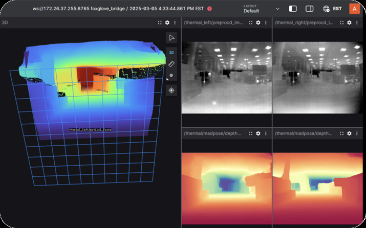
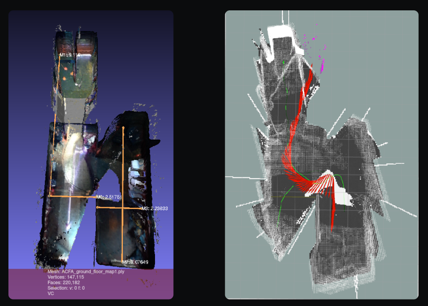
Dense Depth Estimation from Thermal Cameras
Our original depth estimation subsystem uses MoGe to estimate relative depth and MadPose to compute metric depth. The operational workflow is as follows:
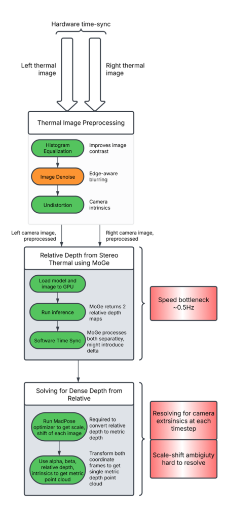
- Time Synchronization: Captured images from the stereo thermal setup are time-synchronized using a hardware pulse.
- Preprocessing: The 16-bit depth data is preprocessed to optimize feature extraction.
- Relative Depth Estimation: The MoGe algorithm generates relative depth maps for both the left and right thermal cameras.
- Metric Depth Computation: The MadPose optimizer computes metric depth using the relative depth outputs from both cameras, leveraging camera extrinsic parameters.
A problem we encountered while using this approach is that the scale varied significantly across consecutive time steps, and as such we were not able to recover consistent local point clouds over time. We theorize that this was because it is an ill-posed problem because the solver attempts to solve not only for the variables mentioned above, but also for the extrinsics. This means that the system can have multiple solutions, and thus, is not a well-posed problem.
We also experimented with cutting-edge machine-learning research for 3D reconstruction such as Mast3r and other algorithms. We did not find success with these approaches either, we theorize that these approaches rely heavily on the semantic appearance of objects in RGB images and utilize priors about their relative positions and sizes to perform 3D reconstruction. These priors do not manifest in thermal images, thus, these approaches trained on RGB images, fail.
The lack of semantic priors in thermal images meant that we had to try classical methods that rely on image intensity features. Classically, depth is calculated from a stereo pair of images by estimating disparity along epipolar lines. In layman terms, nearer objects appear father away in the two images. The distance between the projections of a world point in both images is called disparity. The distance of the object is inversely proportional to disparity. This is what we use to find real-world distances.
Classically, disparity is found using a sliding window approach to find where a pixel and its neighborhood appears in the other image. This location is determined by minimizing the intensity distance between the neighborhood and all candidates in the other image.
This approach did not work with thermal images, because the images are extremely noisy – the images contain time-varying salt-and-pepper noise, which throws off any attempts to compare neighborhoods of pixels.
We were advised to use FoundationStereo for this task of estimating disparity between the images. This is learning-based method that takes in two images and outputs a disparity image. This algorithm has several advantages over the other learning-based approaches attempted above:
- FoundationStereo is trained on multispectral images thus it has generalized to multiple image modalities, including thermal.
- This method does not rely on semantic priors as the other ones did. This is because to calculate disparity, semantic information is not needed, all the information about the geometry is encoded in the relationships between the pixels of both images.
We obtained disparity values from this method and scaled these disparity values to a metric pointcloud as shown in Figure~\ref{fig:foundation-stereo}.
The original model is in trained and inferred in PyTorch. We used TensorRT to accelerate and serialize the model for inference on our image size and on our hardware. We use this serialized model to perform quick inference and are able to publish depth pointclouds at 1Hz.
Points Of Interest (POI) Detection
POI detection refers to the task of detecting and localizing Points of Interest, which in our case are human casualties, so that they can be positioned on the final BGV map, enabling first responders to plan faster rescue paths.
The entire POI detection pipeline operates in four stages:
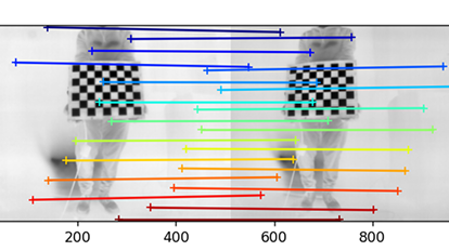
- In-Frame Detection: Human detection is performed on the thermal image feed using a YOLOv11 object segmentation model developed as part of Project HumanFlow at AirLab. The YOLO model has been fine-tuned on thermal datasets collected for the DARPA Triage Challenge and other projects at CMU AirLab, enabling robust human detection on thermal images. The detection pipeline also estimates a 17-point skeletal pose for each human, which is helpful for further 3D localization.
- Cross-Frame Tracking: Once a human is detected, the YOLO pipeline assigns a local tracker to each detection, allowing individuals to be tracked across frames while they are visible in the thermal feed, thereby preventing duplicate detections.
- 3D position estimation: To determine the 3D position of each human with respect to the camera frame, we first estimate the distance (depth) from the camera using a custom approach. We identify the general pose of the human (standing, sitting, or lying down) using the 17-point pose estimation output, and then map the segmented detection area to an approximate distance value using the following approach: – Standing: The segmented area size is mapped to a distance value assuming an average real-world human height of approximately 5.8 ft. – Sitting of lying down: Finely tuned scaling factors are applied to ensure more accurate depth estimation.
- Fusion with odometry heading:Finally, the estimated 3D position (in the camera frame) is fused with the drone’s odometry heading to obtain the final real-world localization of our Points of Interest.
Our final system consistently achieved over 90\% detection accuracy, and its performance was validated across different human poses as shown in the below Figure:

Mapping
Mapping is the task of creating and updating an accurate 3D map of the environment.This will help us in identifying safe routes for the first responders and localizing humans stuck in the environment.
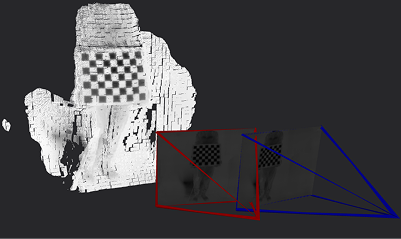
Ground Truth Mapping:
To create a baseline ground truth map of the environment, we used an Intel RealSense camera with NVIDIA Isaac ROS algorithms in a de-smoked environment. This approach enabled us to generate a highly accurate reconstruction of the environment with precise odometry, resulting in minimal deviations from real-world dimensions.
To achieve this we leveraged two Nvidia ISAAC ROS packages:
- Visual SLAM(VSLAM): The VSLAM package was used to generate visual odometry for the drone by utilizing visual features from the stereo IR sensors available on the RealSense camera. To ensure that the IR pattern emitter did not interfere with the visual inputs for odometry, we used the RealSense-splitter package, which allowed us to capture IR and depth frames individually by turning off the IR emitter in alternate frames. This approach enabled us to obtain both IR frames without the pattern, as well as depth and RGB frames, at 15 FPS from the Orin.
- Isaac NvBlox: For mapping, we used the ISAAC ROS NVBlox package, which integrated the generated point cloud with the odometry waypoints from the VSLAM package to create a 3D reconstruction of the environment. From the generated 3D map we extract ESDF slices corresponding to the altitude at which the drone is flying, this enables the generation of traversibility map which can further enable complete drone autonomy. The final map is integrated with 3D human localization.
Indoor Mapping:
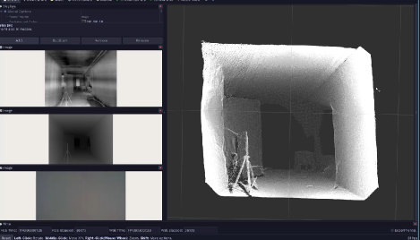
After attempting other approaches, we settled on an occupancy-map voxel based approach provided by the Octomap ROS node for indoor mapping. This node ingests the drone-world origin transformation and the current depth point cloud in the drone’s frame to incrementally update the global map.
The global map is comprised of voxels of a fixed size, which all store the probability that the space in that voxel is occupied. The mapping node also publishes a 2D occupancy map of the environment that displays unoccupied voxels where firefighters can move and occupied voxels which have objects/walls.
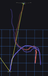
An image of our final mapping capabilities are shown below:
This map is entirely generated on ground control basestation computer and is shown in real-time to the Operator.Further, the trajectory of the drone is overlaid onto the map along with integrated 3D POI localization as shown in the below Figure:

Outdoor In-flight mapping:
As a stretch goal for our SVD Encore demonstration, we attempted
to map the exterior of the building in real time while performing a 360-degree flight around it.
To achieve this, we leveraged our existing RealSense and ISAAC ROS ground truth generation pipeline, while enabling Visual-Inertial Odometry using the RealSense IMU to account for the high motion during flight. We successfully mapped all sections of the building and its surroundings within 8 meters of the drone (the operational range of the RealSense), achieving near-perfect odometry throughout the flight. This can be seen in the below Figure:

Networking
Networking in our system refers to the set of technologies and protocols that enable communication, data transmission, and flight status coordination between the drone and the ground computer over wireless networks.
Hardware
We have at our disposal:
- GCS Air Unit (on board drone)
- GCS Ground Unit (on ground)
- Drone Compute (Nvidia Orin AGX)
- Basestation COmputer (Gigabyte x86 laptop)
Original Architecture
During SVD, we leveraged the optimized HDMI video transmission link on the Herelink radio to transmit a user interface screen rendered entirely on the drone. While this approach helped alleviate bandwidth limitations, it also imposed a high computational load on the Jetson Orin, leading to system instability.
Final Architecture
To address this issue, we first improved the stability of the Herelink radio connection by removing all interfering components operating on the 2.4 GHz band, such as the Orin’s Wi-Fi network card. We then established a unicast Local Area Network (LAN) over the Herelink radio as the sole communication channel between the drone and the ground station. Additionally, we offloaded graphics-intensive tasks—such as integrated mapping generation and user interface rendering—to the ground control computer, leaving only autonomy-critical algorithms running on the drone’s onboard compute. Our final system design is shown in the following diagram:

Our final networking system had the following operational flow:
- Data Transmission: Since we were operating on a unicast network setup that did not support the ROS Data Distribution Service (DDS), we developed custom UDP-based data distribution pipelines. These pipelines enabled reliable transmission of critical data, including drone flight metadata, odometry, human detections, stereo disparity (essential for integrated mapping), and system diagnostics between the drone and the ground computer.
- Thermal Video Transmission: We used GStreamer to transmit a compressed thermal video feed from the drone over the radio LAN. This provided real-time situational awareness and enabled visualization of human detections at the ground station.
- Control: Using the radio LAN, we established a real-time SSH link between the ground station computer and the drone’s onboard computer, allowing low-level control, while high-level drone autonomy was managed through MAVROS topics.
