Fall 2020 Performance
| Requirement ID | Requirement Description | Achieved |
|---|---|---|
| M.P.1 | Register camera-robot coordinate frames with a 10 mm maximum root-mean-square-error (RMSE) | 4.085 mm |
| M.P.2 | Register laser-robot coordinate frames with a 10 pixel unit maximum reprojection error | 5.348 pixel units |
| M.P.3 | 3D scan the surface of the phantom liver in under 5 minutes | 3 minutes and 26 seconds |
| M.P.4 | Segment the liver, including near organ occlusions, at 95% IOU | 97.3% |
| M.P.5 | Generate a 3D point cloud of the phantom liver within 10 mm RMSE when compared with known geometry | 6.34 mm RMSE |
| M.P.6 | Estimate the motion of the phantom liver within 0.5 Hz | 0.055 Hz |
| M.P.7 | Palpate the phantom liver in under 10 minutes | 5 minutes and 27 seconds |
| M.P.8 | Complete the entire surgical procedure in under 20 minutes | 10 minutes and 21 seconds |
| M.P.9 | Detect >90% of cancerous tissue | 100% |
| M.P.10 | Misclassify <10% of healthy tissue as cancerous tissue | 1.69% (For a circularly-shaped tumor) |
| M.N.1 | Comply with Food and Drug Administration (FDA) regulations | Would require FDA-overseen inspection and clinical trials to decide. |
| M.N.2 | Reduce the cognitive overload of surgeon | Requirement satisfied |
| M.N.3 | Not occlude the phantom liver’s visibility to the surgeon | Requirement satisfied |
| M.N.4 | Exit autonomous mode immediately upon prompt | Requirement satisfied |
| M.N.5 | Yield itself to regular safety checks | Requirement satisfied |
| M.N.6 | Cost less than $5000 | Cost $700.90 to build |
We conducted one main experiment for the Fall Validation Demonstration. This involved running our entire system altogether (all performance requirements) and measuring various outputs along the way. We were able to generate a point cloud of the phantom liver with 6.34mm RMSE (M.P.6), which is within our requirements of 10mm. To calculate the RMSE, we fed in the ground truth point cloud of the liver that we had from the CAD model and the point cloud pcd file from the points that we scanned. We then manually align the two point clouds to give the algorithm a better starting point and it runs ICP to align them further.
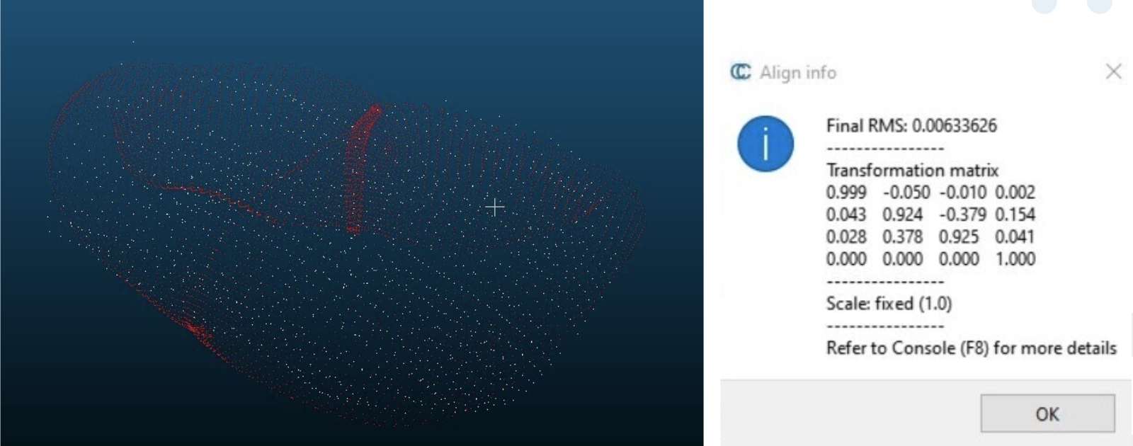
Figure 1: Point cloud accuracy
The second metric we measured was the time it took to complete each part of the procedure. This involved timing the scanning time, the palpation time, and the overall time taken, which encompasses software processing time as well (M.P.5, M.P.7, M.P.8). We timed these procedures with and without injected noise, the results of which are shown in Figures 2 and 3.

Figure 2: FVD times without noise

Figure 3: FVD times with noise
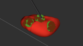
We define tumor tissue in our system as the minimum bounding circle that encompasses all points we classify as a tumor during palpation (M.P.9, M.P.10). We define misclassified tissue as any tissue that is actually healthy that we decide is cancerous based on this minimum bounding circle. Through FVD and FVD encore, we tested various tumor numbers and shapes in order to ensure that our system worked as intended in general cases. The results are shown in the Figure 4 below, Left to Right: 1 circularly-shaped tumor, 1 oddly-shaped tumor, 3 tumors, 1 tumor palpated with noise.
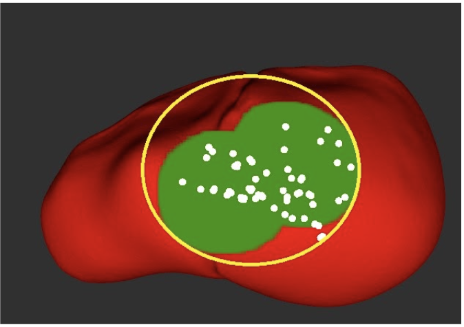
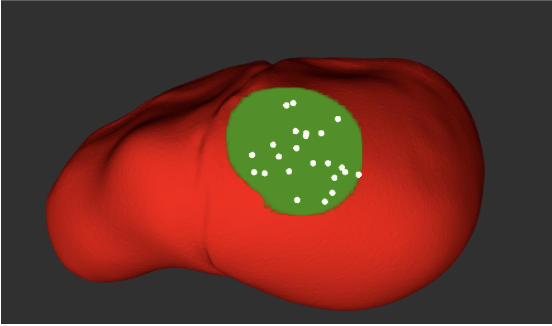
Overall, we were able to meet all of our performance requirements thought our tumor estimation metric (minimum bounding circle) can be improved in the future.
Spring 2020 Performance
| Requirement ID | Requirement Description | Achieved |
|---|---|---|
| M.P.1 | Register camera-robot coordinate frames with a 10 mm maximum RMSE | 4.085 mm |
| M.P.2 | Register laser-robot coordinate frames with a 10 pixel unit maximum reprojection error | 5.348 pixel units |
| M.P.3 | 3D-scan the visible surface of phantom liver in under 5 minutes | 4 minutes and 25 seconds |
| M.P.4 | Segment the liver, including near organ occlusions, at 95% IOU | 97.3% |
| M.N.3 | Not occlude the phantom liver's visibility to the surgeon | Unoccluded view of phantom liver in camera feed |
| M.P.5 | Generate a 3D point cloud of phantom liver with 10mm maximum RMSE when compared with known geometry | 1.188 mm |
| M.P.6 | Estimate the motion of phantom liver within 0.5 Hz | 0.055 Hz |
We conducted four main experiments for the Spring Validation Demonstration. The first was in regards to registration, M.P.1 and M.P.2. The high-level goal of this experiment was to show that our registration algorithms could meet our accuracy requirements. The test for this was performed beforehand because the process is a bit laborious and takes time. We were able to register the camera and robot with a 4.085 mm RMSE as shown in Figure 5 and register the Blaser and robot with 5.348 pixel-unit reprojection error as shown in Figure 6. These two numbers fall within our requirements.
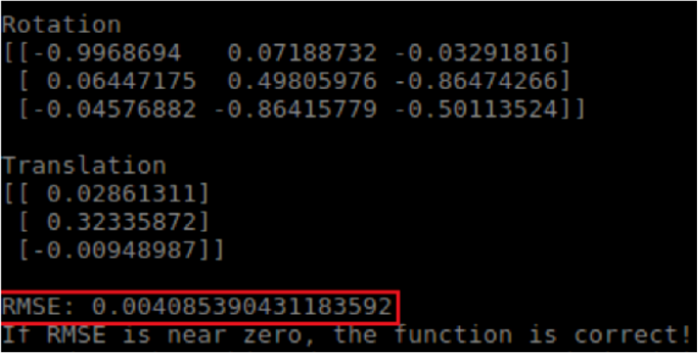
Figure 5: Camera-Robot Registration Results
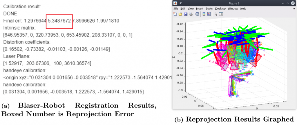
Figure 6: Blaser-Robot Registration Results
The second experiment related to segmentation performance, M.P.4. As stated, we wanted to ensure the algorithm worked under different light intensities. We fed in a video stream from an Intel Real-Sense RGB-D camera of the liver moving on the MSP and calculated the segmented outputs. These were compared to the ground truth frames that we manually labeled. Under different lighting conditions, the current algorithm reaches an IOU of 97.3%. Thus, we were able to satisfy this requirement. An example image from our SVD run is shown in Figure 7.
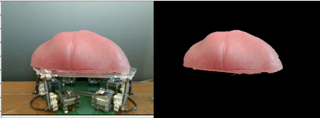
Figure 7: Results of Image Segmentation Algorithm given Image of Liver on MSP
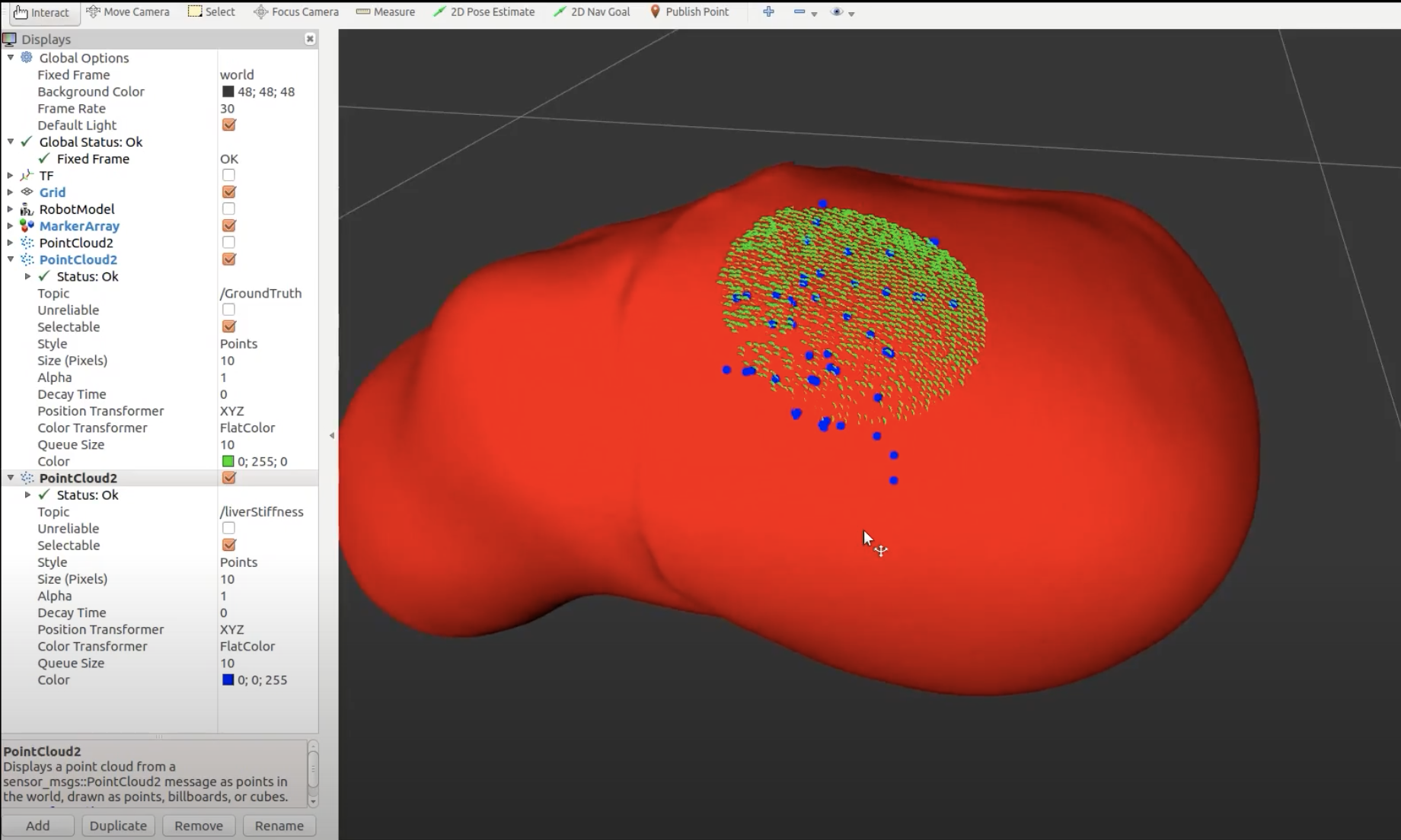
The third experiment we conducted for pertained to M.P.3, M.P.5, and M.N.3, which describe the point-cloud generation. This experiment was conducted on the static liver because we did not have time to test the algorithms with the moving algorithm before we left campus due to Covid-19. We initiated the procedure to scan the visible anatomy of the liver and recorded the point cloud output while timing the procedure. We also checked the surgeon’s camera feed to ensure that the dVRK arms did not block the camera. The partial point cloud that we were able to record has a 1.188 mm RMSE when compared to ground truth, though we did scan the entire liver. The entire procedure took 4 minutes and 25 seconds. Though we were not able to record the entire point cloud of the liver, with the current partial point cloud we believe we can extrapolate to determine that the overall point cloud would have less than 10 mm RMSE. The total procedure time fell within the allotted time from the requirements, so we have satisfied all three requirements. Figure 8 shows these results.
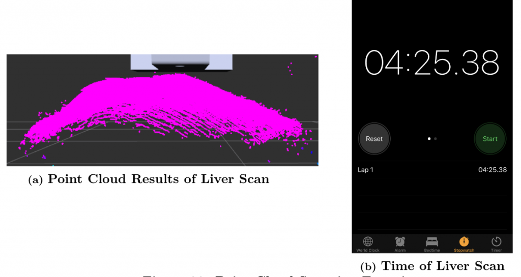
Figure 8: Point Cloud Scanning Experiment
The final experiment was performed to validate \ref{MP6}, the motion estimation accuracy. We set the phantom liver on the moving platform, which was oscillating at different frequencies. Using the Intel RealSense camera, we imaged the moving liver and ran the motion estimation algorithms on this data. The results during SVD are shown in Figure 9. We tested on different frequencies during SVD (0.5Hz and 0.3Hz) and were able to estimate the frequencies within 0.05Hz. This means we have satisfied this requirement as well.
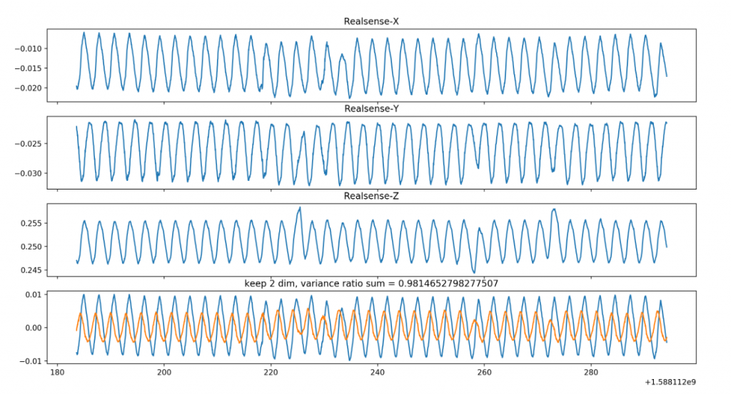
Figure 9: PCA result during SVD, showing estimated movement of the liver along each axis