
Heterogeneous Exploration of Unknown Environments
- In unknown environments, distant obstacles and paths that lead to dead ends are often hard to detect and plan around for AGV sensors.
- We propose a heterogeneous mapping solution that leverages the wide area coverage of UAV to enhance the mapping and localization capabilities of AGV.
- The UAV will fly ahead of the AGV, mapping the environment in front of the AGV, determining obstacles and viable routes, and transmitting this information to the AGV.
- The AGV will incorporate the information from the UAV with its own GPS and LiDAR sensors to localize more accurately and plan a more effective path forward.
Subsystem Details
1. AGV Subsystem
1. GPS based waypoint navigation:
This counts as the basis for the development of navigational capabilities of the AGV. We decided to work on GPS based navigation for the fall semester and extend the navigational capabilities of the AGV by including obstacle avoidance using a LiDAR in to the system. Currently, the AGV has been able to navigate to a given GPS location within a maximum inaccuracy of 3m. For the fall validation test, we gave three waypoints as the navigation goals and the Husky was able to reach all three of them within 3m of the given GPS locations. For the SVE, GPS navigation was removed on the AGV as a more complicated local planner was implemented.
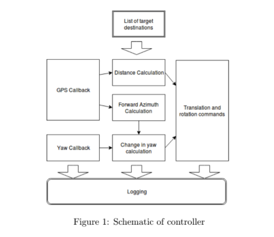
For autonomous navigation, we developed our own GPS waypoint based controller in ROS. The controller reads the target locations one by one from the launch file as a ROS parameter, computes the distance between the current GPS location and target location, orients the AGV towards the target GPS location with the help of an Inertial Measurement Unit(IMU) and then actuates the motor until the distance between current and target location comes under some threshold value. This is repeated for all GPS coordinates saved in the launch file. After reaching the final location, the system enters idle mode.
The schematic of the controller is shown in Figure 1:
2. Mechanical Fabrication
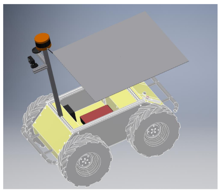
We designed and fabricated specific mounts for the sensors and takeoff platform for the UAV. Figure 2 shows the CAD model for our system.
3. AGV Path Planning and Obstacle Avoidance
a) AGV Obstacle Detection
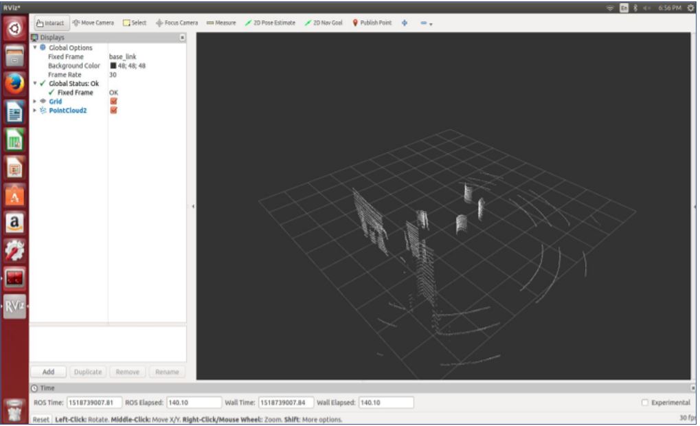
The AGV generates environment map using a LIDAR sensor. A LIDAR usually consists of a scanner and a laser. The laser emits a laser beam at a certain frequency and also receives the reflected laser beam from an object on the path of the laser. This can be used to estimate the distance between the LIDAR sensor and the object by estimating the time difference between the transmitted and received laser. This method is a very reliable method of estimating the distance up to a certain limit depending upon the LIDAR specifications. We have selected Velodyne VLP 16 sensor due to its excellent online support and reliability. As shown in the figure given below, first one depicts the raw point cloud which we get from the Velodyne, then using the PCL library, we filtered out the obstacles of our interest i.e, which are greater than a certain threshold height and which are in the proximity of the AGV, which is shown in the second figure.

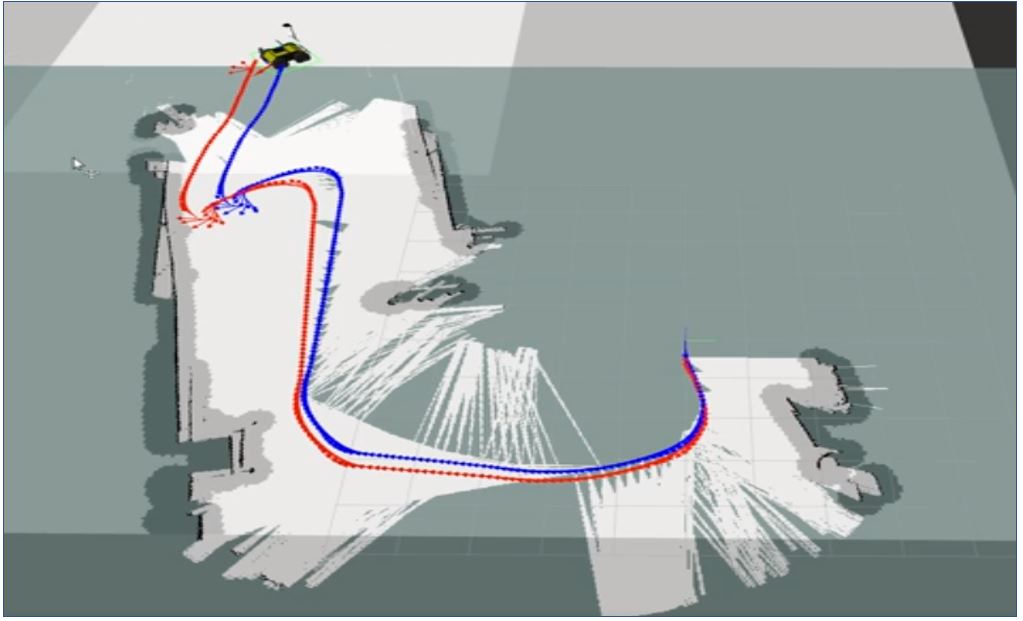
b) Path Planning and Obstacle Avoidance
We used ROS navigation stack for optimized localized-navigation. It uses Search based planning algorithm like A* and has proven to be very effective for motion planning. We integrated GPS and IMU data with this stack for global localization and planning. In addition to this augmenting this system with the input from the Velodyne, helped us in developing a complete obstacle detection and avoidance system. We were able to demonstrate that our system is able to detect and avoid, static as well as dynamic obstacles.
For the global level of path planning our final system was able to record the GPS location given by the UAV on the waypoint navigation text file. The husky navigation stack was reading that file sequentially and executing the path goals provided by the UAV. Two figures given below show the husky navigation with and without obstacle avoidance.
2. UAV Subsystem
1. GPS based waypoint navigation:
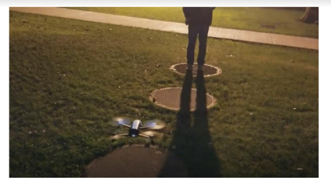
Similar to the AGV navigation, we developed our own controller for autonomous navigation of the UAV. Currently, the UAV has been able to navigate to a given GPS location within a maximum inaccuracy of 5m. For the fall validation test, we gave three waypoints as the navigation goals and the bebop was able to reach all three of them within 5m of the given locations.
Figure 3 Shows the controller design for autonomous navigation. Figure 5 depicts the UAV performing autonomous navigation.

3. CPU subsystem
1. April tag detection:
To determine the traversable paths for the Husky it is essential we are able to recognize those paths through April Tags from UAV’s camera feed. We are able to successfully detect all the april tags in the range of the drone’s camera. The fall validation testing was done with 10 april tags placed within a 2m radius circle and drone hovering at a height of 5m. The detection was shown by overlaying red circles over the april tags and also by displaying them in rviz.
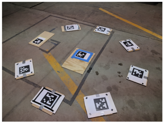
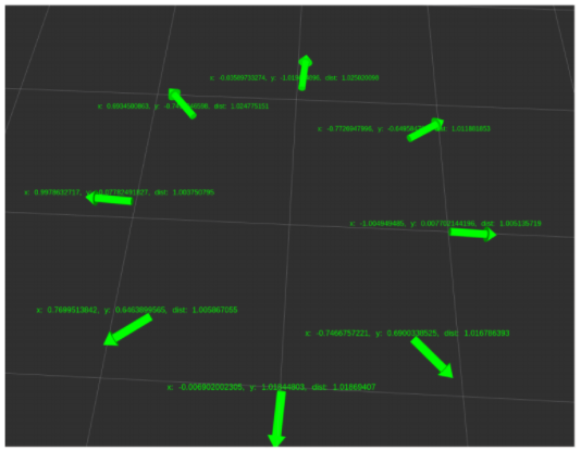
2. Localization of April Tags with respect to a home frame:
We are able to localize april tags with respect to each other with a maximum inaccuracy of 10cm. This is much better than our performance parameter which was 30cm. This test was done with the drone hovering at a height of 5m. The distance was shown by manual measurement between the tag centers in comparison with the computed distance in rviz.
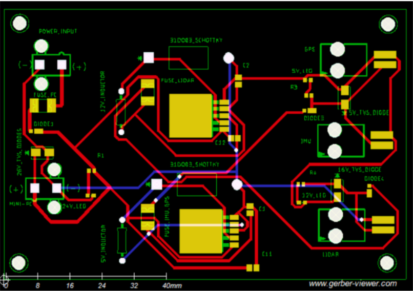
4. Power Distribution Board
We have designed and developed a power distribution board for our system. The board provides Stable voltages to run two 5V devices (GPS and IMU), one 12V Wi Router and a 24V Mini-PC.We are getting nominal drift of 6% from the specied voltages that lies within the operating ranges of the devices we will be using. Since we already have stable DC output from the built-in DC-DC converters in AGV with less than 2% drift, we plan to use our power distribution board as a backup and for indoor testing.
Figures 7 and 8 show the schematic and photo of the PDB during Fall Validation Experiment.
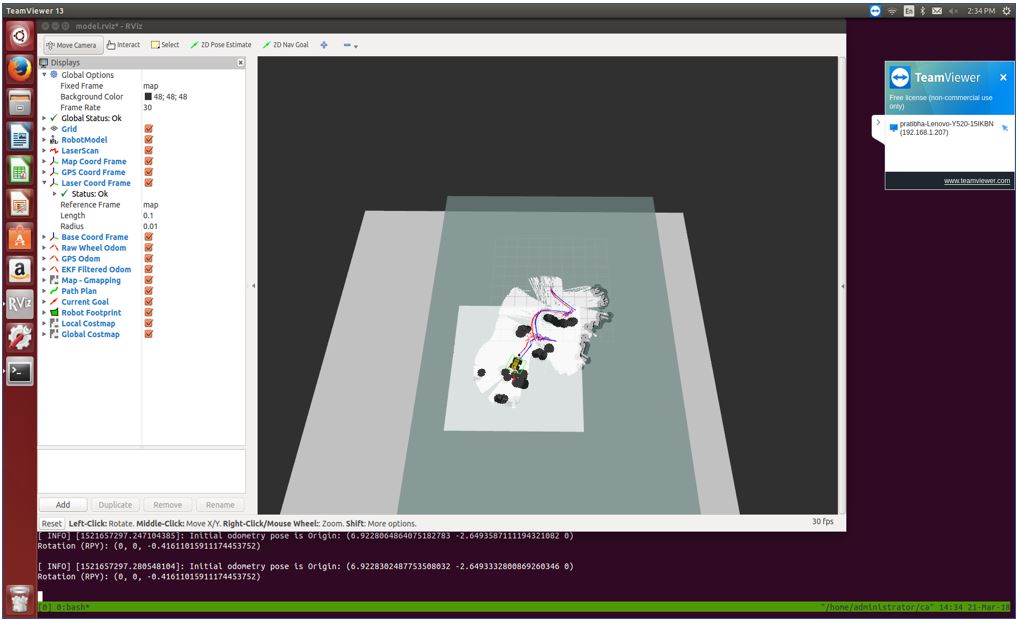
5. April Tag Graph
After detection of the April Tags, we use an internal graph representation as the map for the environment. Specifically, based on the locations of the April Tags, we have a graph of valid “nodes” that represent areas where there are no obstacles. These are key locations that the Husky can travel to. The edges between the nodes are paths that allow the Husky to move from one location to another. As the drone explores further, certain branches will expand more while others are dead ends that get pruned. Below is a visualization of a simple graph that is constructed in RVIZ with tf. Much more complex graphs are present for the SVE.

5. Exploration and path-finding algorithm
Based on the constructed graph, the UAV explores unseen areas of the map to find a valid path to the goal. It does so by finding the closest unexplored April Tag (node) to the target destination and exploring around that area. Based on our specific environment, we can guarantee that any successive April Tag will be within 3 meters to the previous one. At a 10m hovering height, our algorithm is extremely reliable at finding a path if a path exists.
The UAV is not constrained by ground obstacles and so it can directly fly over to any node that it wishes to explore. The same cannot be said for the Husky which must navigate along the vertices of the graph. Based on our graph, finding this path can be solved by a graph exploration algorithm such as A-star. This is exactly what we did. We mark the node closest to the Husky as the starting node, the node closest to the target as the goal node, and we run A-star on the graph with distance as the cost. A high-level depiction of the entire system algorithm is shown below.
