Functional Requirements

FR1. Take input from the user
FR2. Perceive drivable area during navigation
FR3. Autonomously localize itself
FR3.1. Along Row
FR3.2. Correct Row
FR4. Autonomously switch between rows of the field
FR5. Collect visual data
FR6. Identify signs of disease
FR7. Identify pests or signs of pests
FR8. Generate meaningful reports
FR9. Communicate (reports) to users

Performance Requirements

MR1. Autonomously localize itself
MR1.1. In the correct row with 80% accuracy
MR1.2. Cross track control error < 3 in within the row
MR2. Autonomously switch between rows of the field with 80% success rate
MR3. Collect visual data with 75% usable images
MR4. Identify signs of disease on plant with precision and recall > 80%
MR5. Identify pests and /or signs of pests with precision and recall > 80%
MR6. Generate meaningful reports within 24hrs of collection
MR6.1. Label row with plant name
MR6.2. Label image with severity level
MR6.3. Allow user to see and change the severity level
MR6.4. Show date of monitoring on the GUI

Non-Functional Requirements

MN1. Fit in the row of width 24in
MN2. Accommodate various control modes via kill switch and joystick
MN3. Have sufficient battery life to complete a run of Rivendale brassica field
MN4. Not damage plant during navigation

Functional Architecture

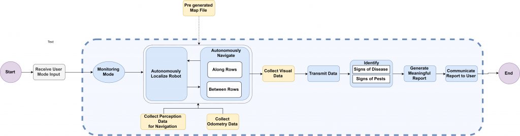
The functional architecture has been simplified to only a single monitoring mode. In this operation mode, the robot localizes itself in the field and then uses the location and a pre-built map to navigates through the field. The robot collects visual data which it processes later to identify signs of pests and disease. In the end, meaningful reports are generated to communicate to the user information about crop health.

Cyber-Physical Architecture

The following figure shows the overall cyber-physical architecture of the robot which has been primarily divided into components which include User Interface, Processing, Sensing and Output. The high level cyber-physical breakdown of each subsystem has been done below (further breakdown is discussed as part of each subsystem).

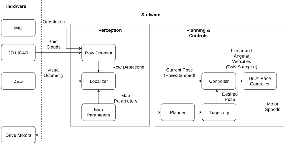
The navigation subsystem is used in both operating modes. It inputs information from 3D LIDAR (Velodyne VLP16 Puck), an Inertial Measurement Unit, and a stereo camera (ZED). The IMU and LIDAR are interpreted by a row detector, which is fed into the localizer along with visual odometry from the stereo camera in order to output the robot’s pose. The map (GPS points at the beginning and end of each row) are passed through a global planner which outputs a trajectory. The robot’s pose is then matched to the trajectory pose using a pure pursuit controller.

Within the monitoring mode, the monitoring subsystem takes images from the robot’s active lighting stereo camera and passes it through a perception pipeline to identify areas of pest and disease. The pipeline includes segmentation via Mask RCNN and depth filtering, both of which are fed into a logistic regression to generate a classified output (in terms of disease and pest severity).

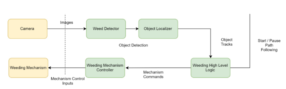
The weeding subsystem uses the stereo camera to collect visual data and location data for detecting weeds in that particular position. After the weed is detected, the 3D location of the weed in the robot frame is calculated and sent to the weeding controller. The weeding controller drives the motors of the weeding mechanism to perform the operation. Higher level mission logic is utilized to confirm the success of the operation before allowing the robot to continue navigation.

System Design

Navigation

Navigation: Overview

We pivoted our navigation strategy which originally required a geometrically consistent point cloud computed via laser-odometry based SLAM to be fitted with a Gaussian mixture model in order to create a sensor model for particle-filter based localization. We instead have used the inherent structure of the farm to converge on a strategy where a row perception module detects row lines in point clouds, and the sensor model is based on computing the probability of a particular row detection given the expected row lines from a list of globally located row lines in the field. This method is far simpler than the prior approach and has the advantage of needing only the row detection module to be changed to accommodate a new environment.

 

Navigation: Row Detection

The row detector is responsible for translating 3D laser scans into row lines. We chose to use the Hesse normal form of a line, in which a line is represented by its normal n and perpendicular distance to the origin d. Points r which lie on the line are therefore defined by r · n = d. The normal n can equivalently be represented by θ = atan2(ny, nx). This parameterization was chosen over the standard in order to represent vertical lines correctly and prevent numerical instability.

 

Navigation: Localization

The localization for the robot, both inside and outside of the row is done using a particle filter. The particle filter is comprised of three main steps which are the prediction, update and resampling steps. For the prediction step, the motion model [1] takes an initial estimate of the pose of the robot using visual odometry from the ZED camera. The relative change in translation (x,y) and rotation (yaw) is calculated and uncertainty is added to this. The uncertainty is sampled from a triangular distribution. For the update step, the measurement model utilizes the row detections and computes a posterior probability of the robot being in a particular pose with respect to the row given this particular row detection P(Z/X). Uncertainty in row detections for distance and angle to the rows is sampled from a Gaussian distribution. For the resampling step, the systematic resampling algorithm [2] is required, where new particles are sampled around old particles which had higher probability.

 

Flowchart for Localization

 

Navigation: Planning & Controls

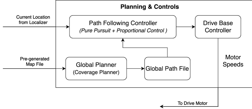Flowchart showing planning and controls pipeline

Planning

The robot should start from a designated starting point, enter the first traversable row and then switch rows to go to the next one. It should repeat this process to cover all the rows in the field.

A coverage path planner was developed which identifies the order in which the rows in the field should be traversed. The algorithm takes the input as the coordinates of the start and end points of the traversable rows from an RTK GPS. These points are then rotated and translated so that the origin is at the start of the first row, x-axis aligns with the first row and z-axis points upward.

Next, the order of traversing rows is identified. The planner is subject to the following constraints while planning the global path

1. Cover entire Area: The robot should cover the entire field of interest.
2. Traverse each row in both directions: Since the stereo camera is mounted on only one side of the platform, the robot needs to traverse each row in both directions so that the plants on each side of the row are captured.
3. Account for Turning Radius: The robot utilizes a skid-steer mechanism and has a large wheelbase. Hence it has a large turning radius. The planner should account for this while making the plan.

The robot should be able to switch from the first to the second traversable row. In case the distance between the traversable rows is less than the allowable turning limit of the robot, the robot skips the row and switches to the next one. Also, the robot does not repeat going through a row in the same direction twice. Finally, we get a list specifying the order in which the robot should traverse the various rows.

This order is converted into a path by generating a rectangular path while switching rows and a straight path for motion along a row.  This path is then discretized in small steps of approx. 0.1m and is passed to the controller as a npy file.

Controls

The control sub-system takes the global path from the planner and current location from the localizer as input and utilizes a control algorithm to track the specified path. Since the robot is a skid steering robot, at any instant the robot can have a velocity along the angular and forward direction only. The sub-system utilizes a proportional controller to calculate the desired linear velocity and utilizes a pure pursuit algorithm to calculate the desired angular velocity of the robot.

Given its current position and orientation in the field frame from the localizer, the controller uses the pre-generated map file and finds the farthest point within a lookahead distance which is in a similar direction as that of the robot. This desired location is transformed to the robot frame. This goal position in robot frame is used to get the forward velocity using a proportional control using Eq. 1 and angular velocity using a Pure Pursuit controller using Eq. 2 with a lookahead distance of ~1m.

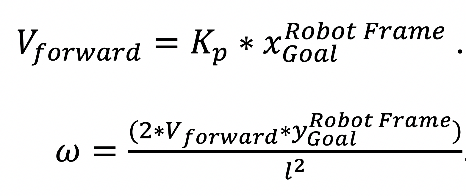These velocities are then transmitted to the drive-based controller.