User Interface
The user interface was implemented using the Google Maps API and Google App Engine. The user interface includes a front-end HTML interface and a back-end python server for tracking regions, way-points, and obstacles.
The UI displays the position of obstacles on the map as well as the real-time position of GroundsBot. The blue polygon on the map represents a hard safety boundary to ensure mowing regions are kept within a specified region. The white polygon is the inputted mowing region. The red lines represent the mowing path planned for GroundsBot.
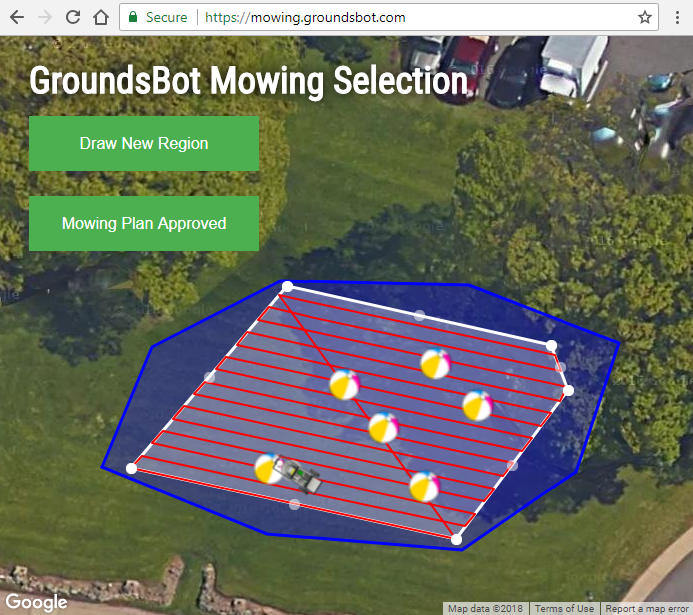
Web interface UI for mowing region selection and mowing plan approval.
Mowing Platform
Chassis
The mowing platform consists of the drive system and the mowing deck. The drive system is a three wheel differential drive platform custom-made by the team. The drive-system consists of two 180 Watt motors and a 10 Amp-hour battery that will allow GroundsBot to operate up to an hour in driving and 45 minutes mowing. The cutting deck is taken from a Worx 770 electric push mower. For safety reasons, the mower blade has been removed from the mowing deck until the team is ready for mowing validation in the Spring. Below is an image of the fully assembled chassis.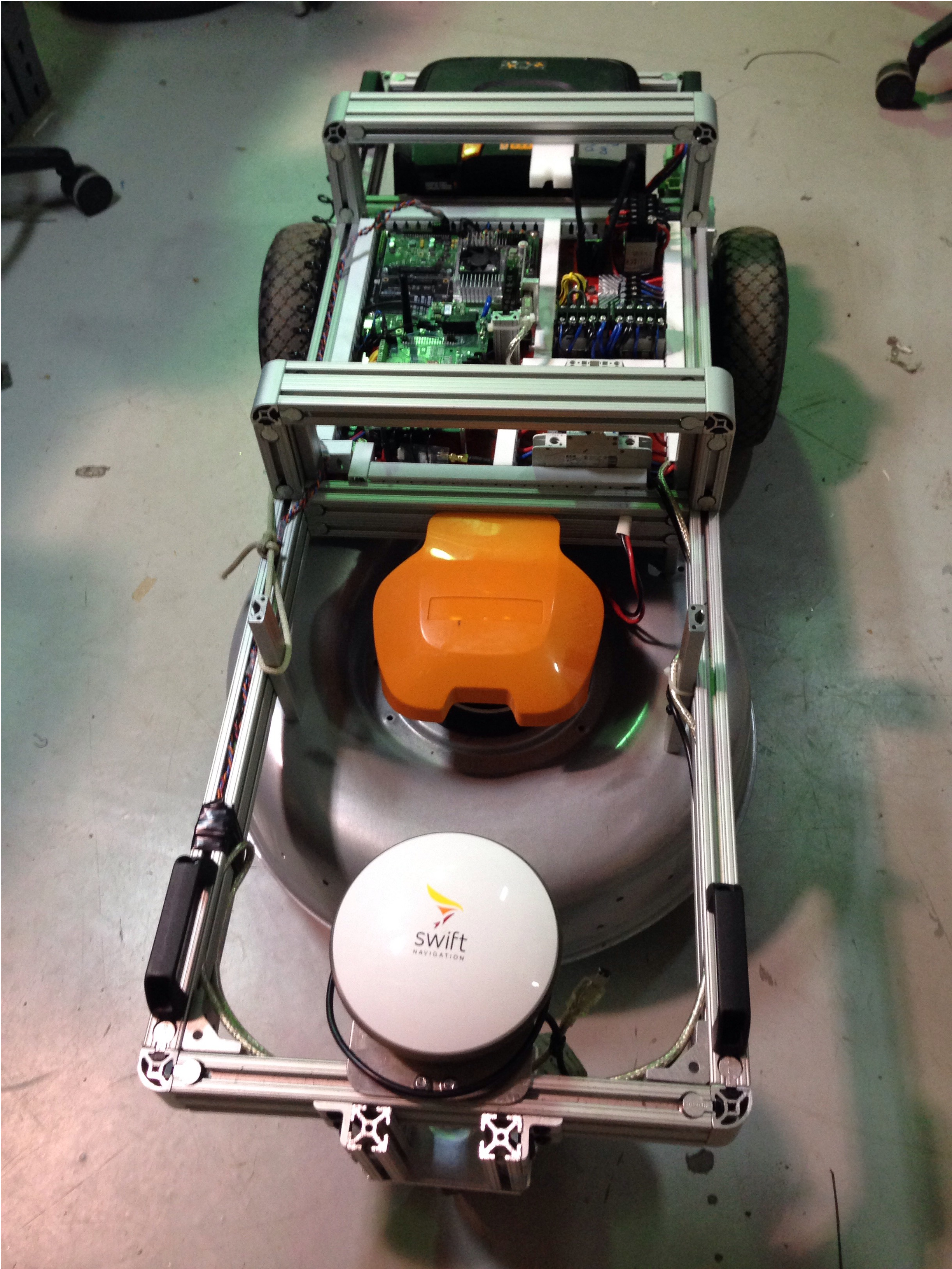
Electronics
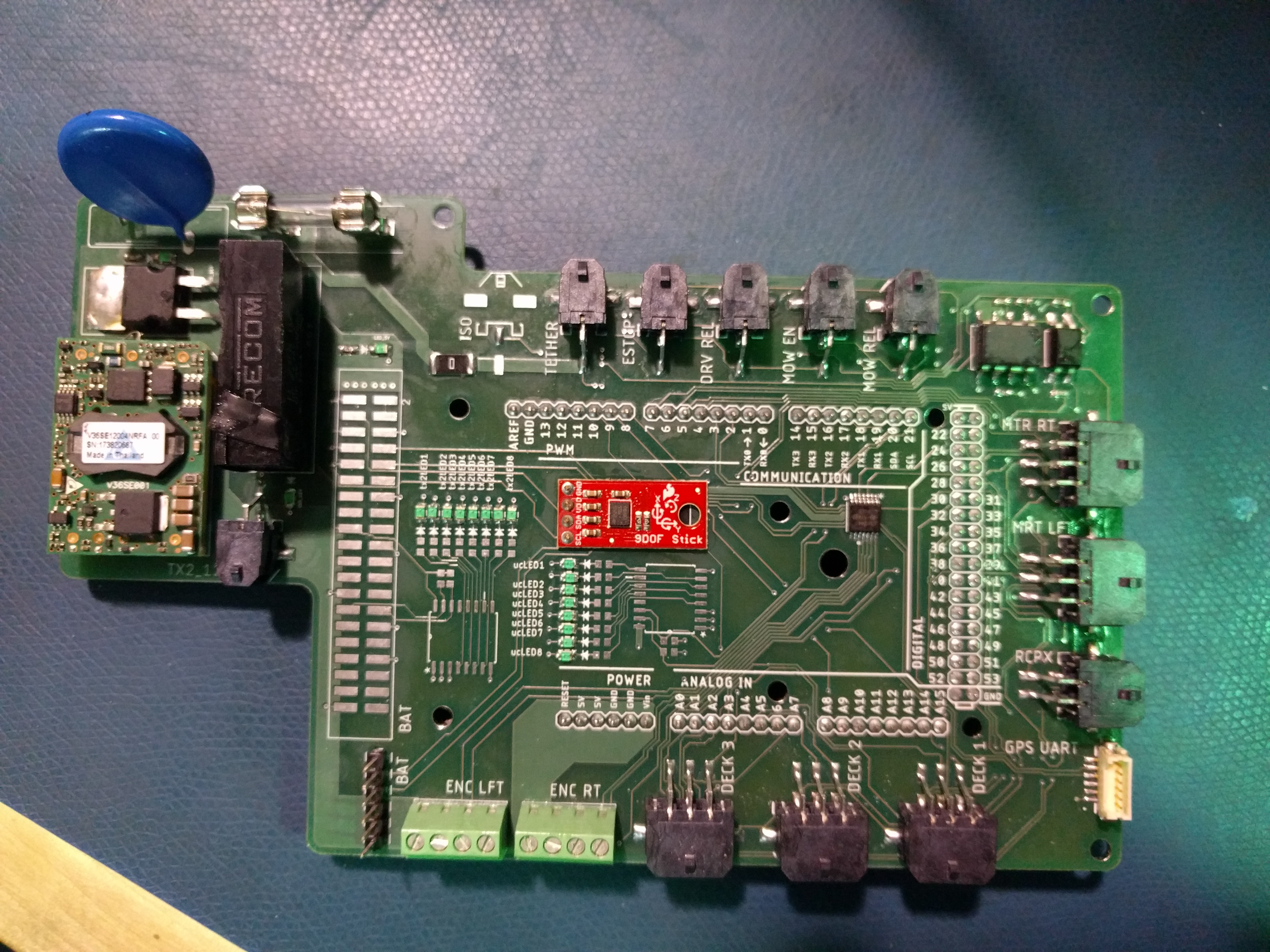
The electronics system powers consists of a high-power system, which powers the motors and mower, and a low-power system, which powers the Jetson TX2 and the Arduino as well as necessary sensors. The low-power distribution system is managed with a power-distribution board that acts as a shield for our Arduino Mega. This power-distribution board is responsible for providing connectors from the Arduino to the Jetson TX2 and other sensors as well as providing protection and power to the Arduino, Jetson TX2, and sensors. Because of the specific and unique requirements of the power-distribution board, the board was designed and assembled by the team. Below is the final result of the power-distribution board.
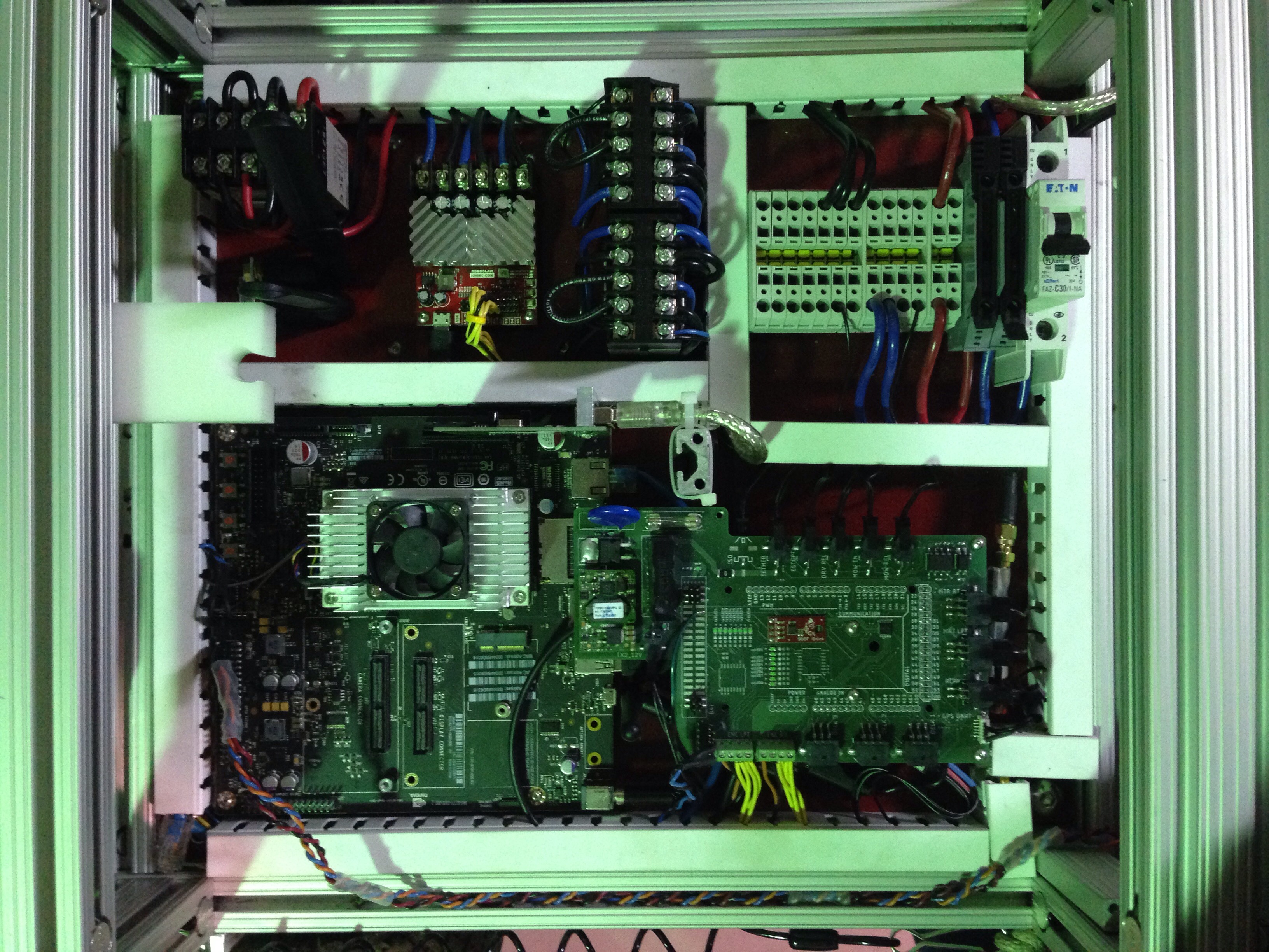
The high-power distribution system was implemented with a series of relays that can be controlled by the Arduino and a set of fuses to manage over-current and over-voltage protection. The high-power system also contains safety mechanisms to stop GroundsBot immediately if a kill signal is sent. GroundsBot currently has two kill signals. An RC controller is connected to the Arduino to manually control GroundsBot and send a send a kill signal if a switch is triggered. A physical kill switch is also included. GroundsBot has a tethered switch in line with the power-distribution system. If the tether is pulled, the line to power GroundsBot is opened immediately shutting down the robot. Below is the final result of both the high-power and low-power systems integrated on GroundsBot.
Perception and Mapping
The perception & mapping subsystem is responsible for using lidar scan data to detect obstacles and generate a costmap to be used by the navigation subsystem.
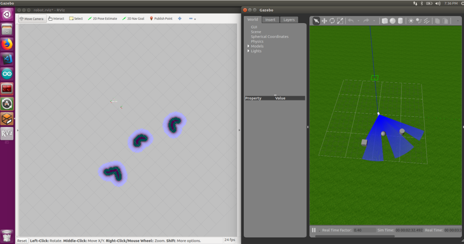
Obstacle detection starts with a laser scan from the Hokuyo UTM-30LX lidar. This planar lidar generates a 180 degree laser scan that identifies the distance to any obstacle seen. The laser scan is filtered using a median filter to reduce the amount noise in the scan. The laser scan is read in by ROS navstack’s costmap2d node. This node populates a costmap of obstacles from the laser scan. The costmap is then used by the navigation subsystem to generate a plan to avoid obstacles. The figure above shows a costmap on the left being populated in simulation on the right. Notice the areas of black in the costmap that correspond to obstacles in the simulation.
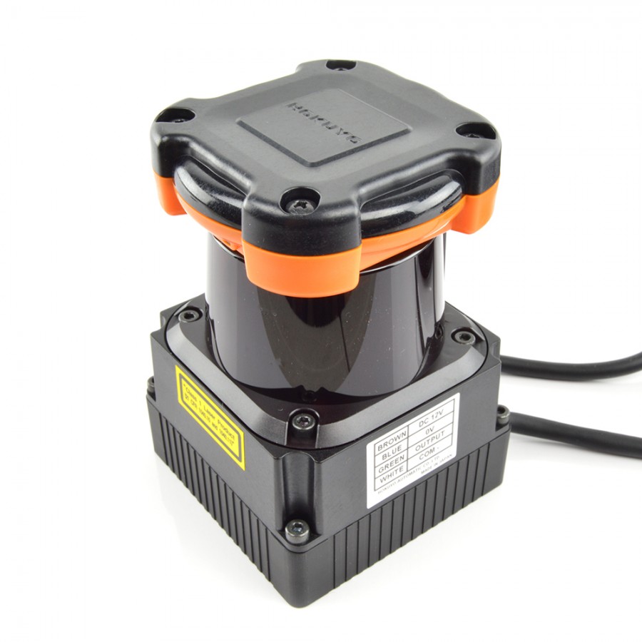
UTM-30LX LiDAR used for obstacle detection.
Navigation
The navigation subsystem receives a coverage area and sensor input, then sends commands to the motors to ensure GroundsBot covers the entire input area. This task can be split into five key activities: localization, coverage planning, waypoint serving, global planning, and local planning. These activities are separated into ROS nodes that work together to make up the complete Navigation subsystem. Let’s take a dive into each activity to learn the specifics of how they work.
Localization
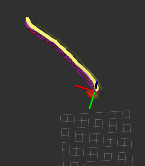
The localization node reads in data from the IMU, RTK GPS, and wheel odometry, then uses the data to estimate the robots pose. The pose estimate is generated by an extended Kalman filter that fuses acceleration and orientation information from the IMU, wheel velocities from the wheel odometry, and absolute position corrections from the RTK GPS. The node is implemented using the ROS localization package. It’s also important to note the IMU data is fairly noisy from the direct sensor, so a complementary filter is used to produce smooth readings. The figure below shows the localization node estimating the position of GroundsBot as it moves around. The final pose estimate is critical for planning an accurate path toward the goal.
Coverage Planning
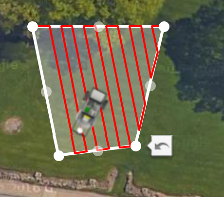
The coverage planning node accepts a polygon drawn via the user interface and returns a set of GPS waypoints, which the robot will follow, in a zig-zag pattern covering the entire input area. The plan minimizes the number of turns required by GroundsBot to cover the area by slicing the polygon along the direction of the longest side. The figure below shows the zig-zag coverage path generated by the node. Once the polygon is sliced, a list of GPS waypoints are returned for visualization on the UI. When the points are approved, they are sent to the waypoint serving node to send waypoint goals to GroundsBot.
Waypoint Serving
The waypoint-serving node reads in this set of GPS waypoints and publishes a target waypoint for the planning node to subscribe to. The node keeps track of all the waypoints GroundsBot has visited and increments through the list in order, publishing a single waypoint at any given time. This published waypoint is then used by the global planner to generate a target path.
Global Planning
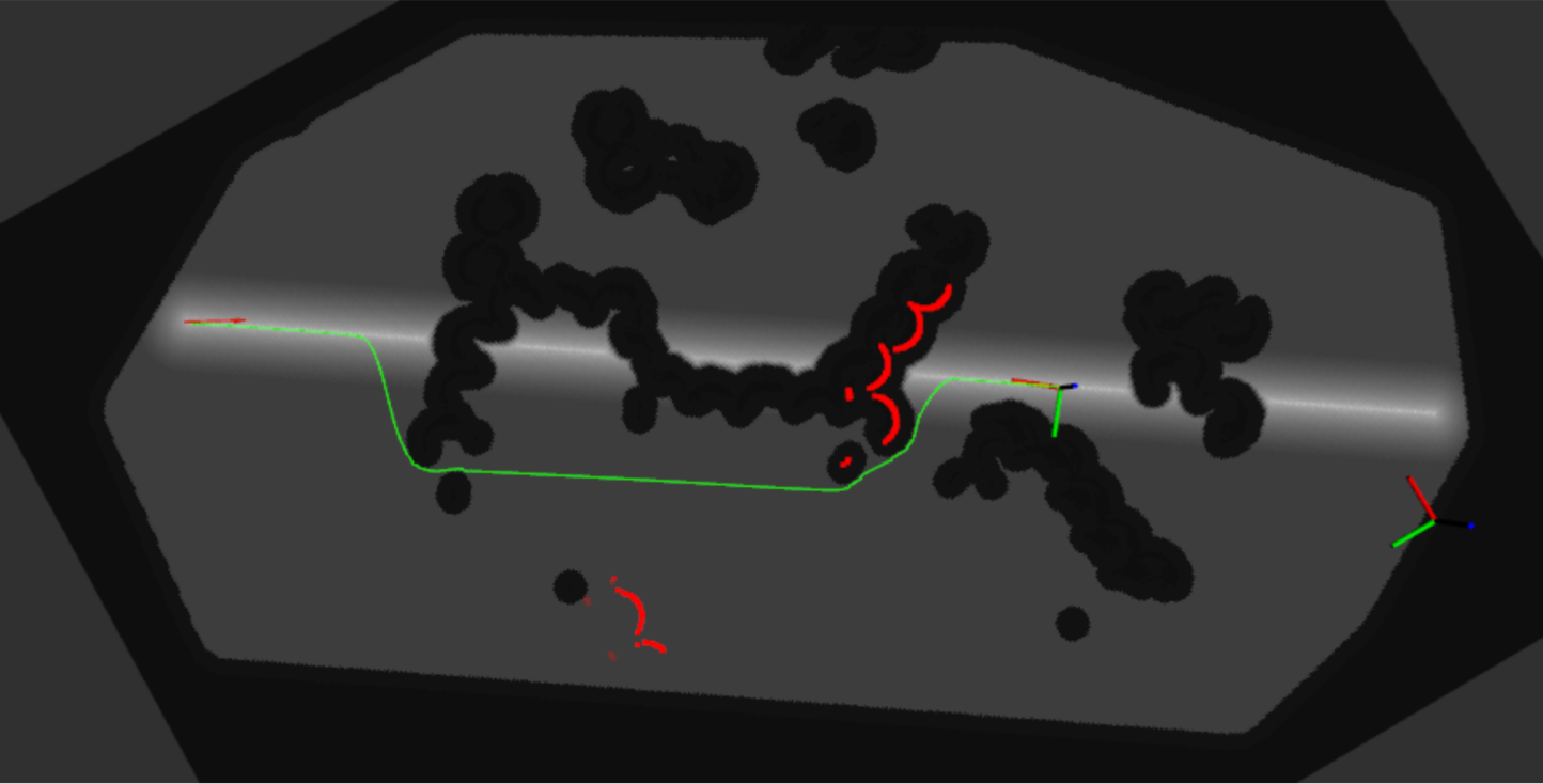
The global planner brings together the pose estimate from the localization node, the target waypoint from the waypoint-serving node, and the costmap containing obstacle information from the perception subsystem. The costmap, however, is not in the necessary format. The costmap is modified to provide rewards (less cost) along the direct line from the last waypoint to the next waypoint. This creates a behavior that attracts GroundsBot to stay on a straight line and navigate along the edges of obstacles. The figure below shows the line drawn on the modified costmap. The modified costmap is then used by ROS navstack to generate a global plan. Navstack uses Dijkstras algorithm to find an optimal path to the target waypoint. Once the path is generated, it is sent to the local planner.
Local Planning
The local planner takes in the global plan and GroundsBot’s current pose estimate, then outputs velocity commands to the Arduino node. The node first gets a carrot waypoint from the global plan. The carrot waypoint is a pose along the global plan about 2-3 meters in front of GroundsBot. This waypoint updates at a frequency of 15 Hz, so it is always a waypoint just ahead of GroundsBot’s current position. The node then uses the current pose published by the localization node and the carrot waypoint to determine a trajectory to move in. Specifically, the node uses two PID controllers to minimize GroundsBot’s yaw error towards the waypoint and minimize GroundsBot’s distance towards the waypoint. The two PID controllers output a forward and angular velocity for GroundsBot to move at.