Overview
We successfully integrated the mobile base, manipulator and sensor and are now in the phase of testing its ability to pick up toys and navigate on different types of floor.
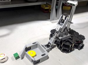
The picture below shows the completed assembly of CuBi that we used for our demonstration. The robot has the Turtlebot 3 Waffle Pi as its mobile base. The base has manipulator fitted on the top layer and has Intel RealSense and Hokuyo lidar mounted on it. It has a PCB for power distribution and an OpenCR controller that is used for the mobility of robot. The system is complete and functional, and we will improve the design for robustness and performance in the coming semester.

The initial robot URDF was developed with modularity to make it easier to add more features as we build the robot. Currently, it contains the base and the camera mounted with the various transforms published and visualizations with rviz.

The state machine that is depicted above is used by CuBi to perform its entire operation. When CuBi is turned on it goes on to ‘search mode’ when it performs a 90 degree sweep in either direction till it detects an object. Once an object is detected, CuBi switches to ‘pick-up object mode’ when it moves to the goal pose, picks up the object. Then in the ‘drop-off mode’ it goes to the home position to drop the picked object on the tray. Then it resets to the home position and starts searching for an object. The state-machine also switches to Back-Off state in case either an objects gets trapped between CuBi paddles or the computer vision of the tray detects that no object was successfully picked-up.

Mobile Base & Mobility
We have performed trade studies on various available off-the-shelf mobile robot platforms, as well as the option to build our own mobile base from scratch. Then we chose the TurtleBot 3 Waffle Pi as our mobile base platform. The main reason to select this platform is the high- modularity design and capability to be easily modified and integrated with other components.
During the past semester, we have finished the assembly of the entire robot. The base is powered by two Dynamixel XM430 motors with a differential drive steering mechanism with two caster wheels on the back. Dual large capacity Li-Po batteries are mounted on the base to power the system, ensuring at least 1 hour running time once fully charged. In the middle layer, an OpenCR microcontroller board is installed to control the chassis motors. It has an embedded IMU onboard, and continuously sends fused IMU and wheel odometry information to the onboard computer through a serial port. On the top layer, we have mounted the manipulator, the NVIDIA Jetson TX2 onboard computer, and the power distribution PCB that we designed.
Currently, both software and hardware components of all other subsystems have been fully integrated together with the mobile base. The base can be controlled either by using a remote joystick, or by receiving velocity commands sent from other nodes through ROS.
Electronics
Please refer to this page.
Grasping
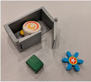
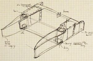
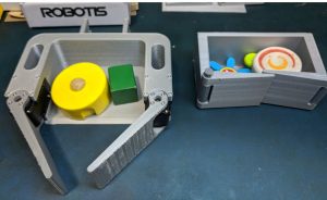
Once we decided on a concept for our robot, we prototyped a simple version of it to validate its grasping. The 3D printing assembly allowed us to see areas for improvement such as the filleted tray base and the overlapping paddles, and overall it was observed that the system is fairly robust and compliant for grasping, since we are using a “caging” grasping strategy.
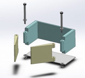

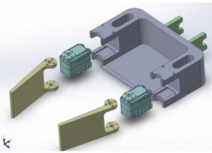
We zoomed in enough mechanical details to validate it conceptually, and transitioned it to a CAD drawing for prototyping of the actual sub-system.

 We increased the tray size to accommodate two tennis-ball sized toys.
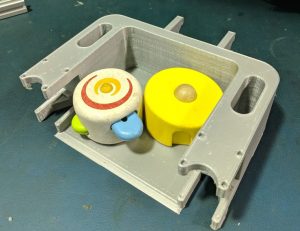
We added provisions for servo-motor wiring.
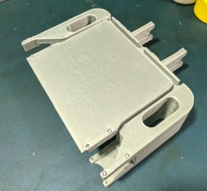
Completed tray compared with first prototype.
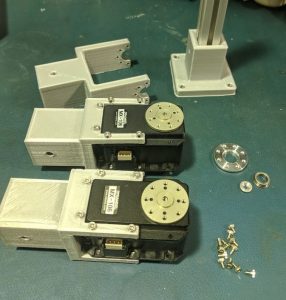
We moved to build the robotic arm by 3D printing the servo-motor brackets and using aluminium extrusion for the links between the revolute joints.
We completed the manipulator and validated for its payload.
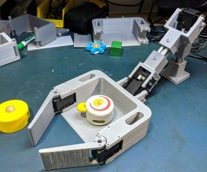
The manipulator is actuated by a pair of Dynamixel AX-12A motors for the gripper and a pair of Dynamixel MX-106 motors for the arm, making it a 4-DOF manipulation system. Each paddle is half the size of the tray which minimizes the possibility of the object getting stuck. The links are made up of 80/20 extrusion aluminum bars, and the brackets and tray are 3D-printed.
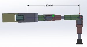
We estimate a maximum estimate weight of 500g for the tray + 2* 100g. For toys, and apply a safety factor to allow for 500 grams of payload. Therefore the total weight for tray plus objects might reach 1Kg, Here we consider the short straight section of the arm to have negligible specific weight.

We then calculated the torque necessary. At its extreme limit, we show the arm of force below, and torque which is:
T = payload * arm_of_force
T = 1.0Kg * 32cm = 32Kg.cm

Finally, we compare it against the shoulder servo motor Dynamixel MX-106 at 12 at the shoulder joint: 8.4N.m = 85.6Kg.cm
Therefore our maximum torque required would be 32Kg.cm / 85.6Kg.cm = 37%
The manufacturer recommends that for smooth motion, that we should keep the required torque within 20% of stall torque = 17Kg.cm
That would translate to 17Kg.cm / 32cm = 0.535Kg = 535g.
For operation carrying only one toy, we would be within the smooth action spec of the manufacturer, for larger loads we might experience “jerky” motion, but we would be well under the specified stall torque of the motor.
Perception
Work was done on segmentation of 3D data and initial results were obtained. This will be improved and further work will be done to estimate the size of the segmented objects and validate the size of the objects of interest and see the minimum distance to camera, which will aid in camera placement.
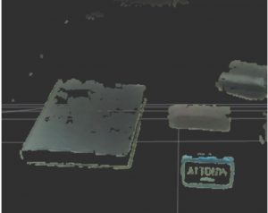
Below is the best output for a very carefully selected 3D image frame. But it is not the case all the time. Work has to be done to make a good pre-processing output for almost every frame and object.
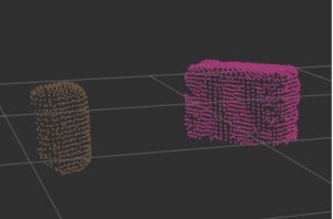
Fit oriented 3D bounding boxes on the objects with their pose and dimension estimates relative to base of the robot. We get a lot of false positives and this will be improved.
A stereo RGBD camera is used for obtaining rich visual RGB data for classification, as well as depth and point cloud for size and distance estimation. Combined information is used to estimate the size, pose and type of object.
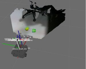
A combination of techniques such as geometric vision, learning-based and probabilistic methods are used to classify objects into two categories: objects to pick and obstacles to avoid. The picture below shows how are perception pipeline works in real-time.
Currently, classical vision techniques and PCL library is used to process the point cloud. A region of interest is cropped, noisy points are removed, RANSAC plane segmentation is performed, followed by clustering of remaining objects on ground.
A 3D bounding box is fitted around each detected object and the pose is estimated to classify them according to threshold criteria of position and size. Finally, object tracking is applied to uniquely identify these objects over time.
To complement geometric features, learning based methods with additional labeled or synthesized data will be used. This will also aid in obstacle detection. A list of detected objects with their absolute positions in the map (calculated with the help of relative positions with respect to the robot) will later be maintained and utilized by the planner for navigation.

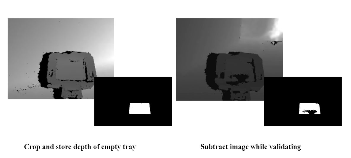
To identify whether a pickup is successful, we developed a vision-based validation pipeline. The following describes the pipeline for pickup validation. The manipulator is commanded to go to the fixed validation position on boot up. Then the depth image of the empty tray is collected and stored. After getting the pre-defined corners of the region to crop, this cropped portion is warped with inverse perspective mapping and rectified for better comparison. Then the current depth image is obtained when the comparison is required as shown in the figure below. The same procedure is followed as the empty tray. Now for comparison, the difference of the depth images of the cropped regions in both can be used against a threshold to validate the presence of an object in the tray.
Mapping & Localization
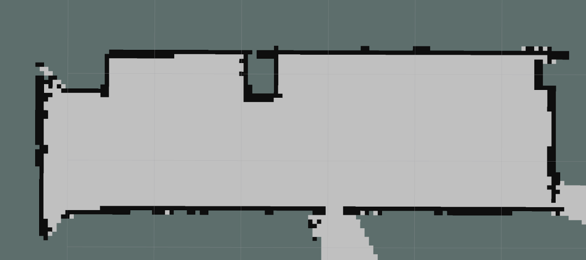
In order to operate robustly in the environment with a potentially unknown starting location and the ability to recover from odometry drifting, CuBi must-have essential information regarding the environment. With the Hokuyo URG-04LX-UG01 LiDAR installed, CuBi is able to map the environment beforehand, and use the map to localize itself afterward by matching the laser scans to the map.
The LiDAR gives us a continuous stream of range reads up to 6 meters, forbearing angles between -pi/2 to pi/2 for every 0.3-degree increment. With that data stream, we use Hector-SLAM[8] package to create a map of our environment. After successfully building the map, it will be saved to the hard disk of CuBi’s onboard computer. We then use the Adaptive Monte Carlo Localization (AMCL)[9] package, which essentially uses a KLD-sampling approach with a particle filter, to track the pose of the robot with respect to the known map. In the particle filter, the odometry information of wheel encoders integrated with IMU is used as the propagated initial guess. The laser scan matching result is used to update the filter. As the particle filter runs, it keeps updating the relative transform of the odometry frame with respect to the map frame, which corrects the odometry drifts.
Our testing proves that CuBi is able to localize itself well in the testing area, with respect to the pre-built map. It is also able to recover and re-localize itself after getting stuck, where wheel odometry may have already drifted with a significant amount. The built map is shown in the figure below.
Planning & Control
The planning and control subsystem consists of an exploration module as the global planner, a local planner, and low-level controllers. The exploration module analyzes the map information and sends waypoints to the state machine. The details regarding the exploration module will be described in the section below. The state machine then interacts with the local planner and controller. The mechanism is described as follows.
The local planner and low-level controllers consist of three layers. The outermost layer receives information from the state machine, the object detection module and the localization module. It utilizes the TF package to query any necessary frame transformations. Any target pose received will be transformed with respect to the map frame, and set as the goal. Once a goal is specified, the middle layer will then compute the relative error of CuBi’s current pose relative to the goal pose. Then it generates a series of motion-defined below. Each motion is tied with a relative error in terms of distance or heading angle. This error is sent to the last layer which uses a position-based PID controller to compute and publish command velocities to the base motor controller board.
The middle layer of the local planner will generate CuBi’s motion as follows::
- Rotate to orient directly towards the target position
- Move straight forward along the x-axis of the base frame to approach the target position
- Rotate until reaching the target orientation
In addition to the control of the base, the state machine also interacts with a node that controls the Dynamixel motors of the manipulator. The manipulator has a fixed set of configurations, such as moving, pick-up, drop-off, pick-up validation, box-approaching, etc. The entire pipeline is integrated using the Robot Operating System (ROS). The availability of ROS packages for Dynamixel motors and the Turtlebot base proved very beneficial to our cause.
Exploration
For exploration, the goal was to create a pipeline that was as flexible as possible. We wanted it to be robust to different room shapes and sizes. The major assumption we made was that a room has four main sides that define it.
The exploration module reads in the map and the metadata from the file. The occupancy grid image is very large and the room takes up approximately 5% of it. To speed up exploration analysis, we cropped it to the size of the room. We store how much was cropped, so we can map back the pixels into the original image. We then use RANSAC to find major lines created by the borders of a room. Once the lines were found, we clustered them into two categories using K-Means. We got the two largest lines in each of the groups to define the borders of the room. We later found the edges of the lines to create a convex hull. Finally, we set all points outside of this occupancy grid as obstacles. This border prevents Cubi from exiting the room through the small holes we have around the map. The process of refining and pre-processing the map is general and automatic.
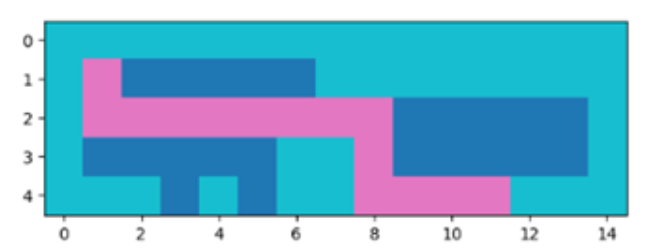
Once the room was defined, we needed to decompose the cells. We restricted Cubi’s range of movement between cells to be forward, backward, right and left. In this way, Cubi always enters the next cell perpendicular to the cell boundary and we can assure that it can scan the entire cell when going to its centroid. We decided the cell size should be 0.7m x 0.7m as Cubi can reliably see toys within a radius of 0.7m. This allows Cubi to scan one cell and parts of the ones in front and to the sides. This extra redundancy was created to ensure we pass through most sections twice.
To create the cells, we decided to use a conservative approach. The resolution of the cells in the stored occupancy grid was 5 cm. We grouped the cells, so they were decomposed into the size we wanted: 0.7m x 0.7m. When grouping the cells, if any of the smaller 5cm cells contained an obstacle, we would label the entire decomposed cell as an obstacle. This conservative approach acted like a way to inflate obstacles. Once we created the decomposed cell grid, we used the centers of all the cells as the waypoint.
As of now, the exploration policy is a very simple one that right followed the walls only visiting unvisited cells. Remember Cubi can only move in four directions. If it was surrounded by obstacles or visited cells, it would go to the closest unvisited cell. The ending condition was having visited all the waypoints. The exploration policy also takes into account the direction Cubi is facing, so that not only is Cubi sent to the right centroid but is also pointing correctly towards the next place it needs to go. Overall, this process allows Cubi to avoid obstacles found on the map and ensure that it has covered the entire room.
Finally, we also optimized our planner algorithm for situations when CuBi had to travel from point-to-point by reducing the number of turns it would take to complete the task.
We were able to succinctly add cost for state transitions between cells where a turn would be necessary. As shown in the figure below, CuBi traverses the same path, but the latter one, turning twice instead of three times. In practice that saves CuBi valuable time when exploring and collecting toys.

Modeling, Analysis & Testing
As a proper system engineering design process, we have been doing a lot of modeling, analysis and testing while designing and implementing our system.
Specifically, for the perception subsystem, we modeled the objects to pick up based on size, which is specified in our system functional requirements. We then implemented and fine- tuned our computer vision algorithm to classify the objects accordingly, with outlier rejection.
For the mobile base subsystem, first we validated our maximum traction that the chassis motors and wheels can provide by testing the robot with payload on different ground surfaces, such as smooth indoor floor surface and carpets. We then adjusted the weight distribution of the system, in order to avoid slipping on smoother surfaces.
We also evaluate the accuracy of wheel odometry, by comparing the reported value to the actual distance measured by hand that the robot travelled, to make sure that the amount of odometry drift was within the range specified in our performance requirements.
For the grasping subsystem, we designed, tested and iterated multiple generations of the paddle design of various length, roughness and shape. Half size of the tray as the paddle length was proven to be the most robust for grasping. Moreover, we estimated the maximum payload required for each joint of the manipulator, and chose motors based on the calculated torque required.
For the electronics system, we calculated the power consumption of all the onboard components. Given the 1 hour running time as one of the performance requirements of our system, we then calculated the battery capacity needed and installed dual batteries based on that.