Fall Semester
Hardware
During our meeting with the sponsor, we scope the project to be without obstacle avoidance. Thus, we remove the D435 camera.
Our final hardware setup consists of the following:
- KUKA LBR Med 7
- Realsense D405
- Vention Table
- Custom EE with Drill
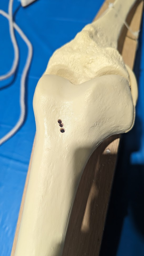
- Bones with Bone Mount
- 3D-printed stencils for verification
Drill Subsystem
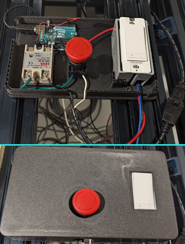
Our drill circuit box was just a floating box without a lid during the spring semester. We accidentally dropped it to the ground during the fall semester, indicating that our floating circuit box is risky. Thus, we redesigned the circuit box and fixated it on the table.
Perception Subsystem
The perception subsystem (which we internally refer to as the ParaSight system) performs multiple functions and is essential to fulfilling one of our core requirements of replacing invasive IR trackers.
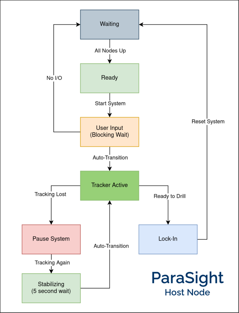
At the center of this system is the Host node – a pytransitions-based Finite-State Machine (FSM) that synchronizes the tracking and registration pipelines and also reacts to inputs from the surgeon IO. The overall flow is depicted in Figure 3, and the description of each state is as follows:
System States
- Waiting:
This is the initial state where we wait for all other relevant nodes to be active (e.g., Realsense, planning stack, etc.). - Ready:
Once all nodes are up, we transition to this state where we wait for the user to start the system. - User Input:
When the user asks to start the system, they are presented with a user interface to annotate points on the femur/tibia. Since this can take a while, this is a blocking wait. - Tracker Active:
Automatically transitions to this state once the points are annotated. These points are passed to the tracking module, which monitors the visibility and stability of these points while tracking them. Whenever the points are stable (i.e., no motion), we run registration to localize and update the drill pose. - Pause System:
If tracking is lost (i.e., the annotated points are no longer visible in the camera’s field of view), we stop publishing the drill pose and pause the overall system while waiting for tracking to be restored. This is done to ensure safe operation of the system. - Stabilizing:
Once tracking is restored, we wait 5 seconds for the system to stabilize before switching back to the active state. - Lock-In:
Finally, when the user is ready, they can give the command to drill, causing the system to “Lock-In”. That is, tracking and registration are stopped to prevent the drill pose from changing while the manipulator moves in to drill. The system then goes back to the waiting state, ready for the next drill.
While the Host node interacts with many subsystems, the main nodes it manages are the Registration and Tracking nodes. These will be discussed in detail in the next sections.
Perception: Registration
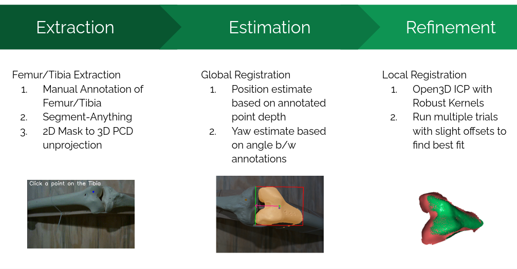
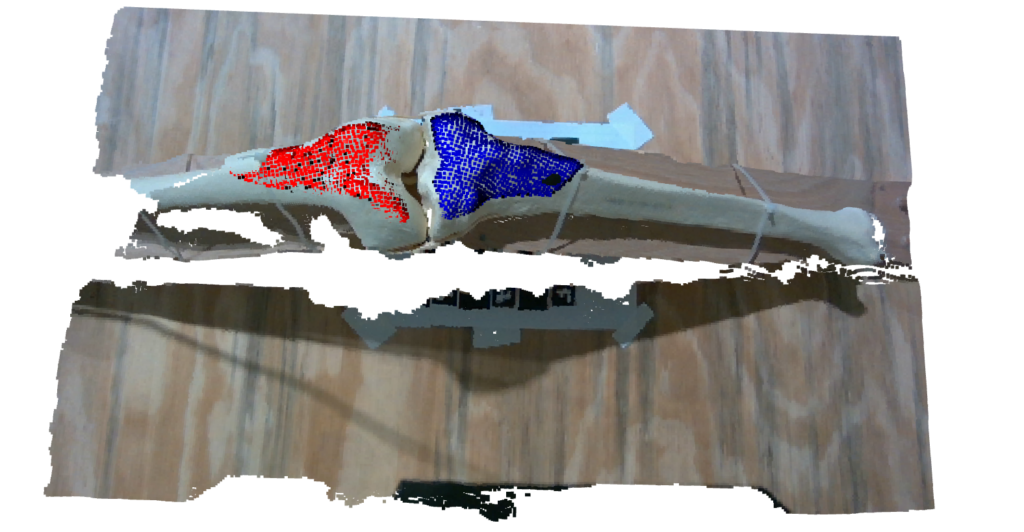
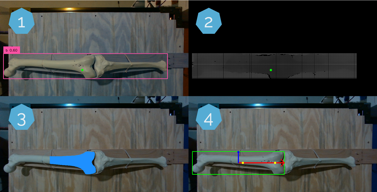
Registration is the process of localizing where the bone (and consequently the drill pose) is located within the scene. We use the Intel Realsense D405 camera mounted at the end-effector to obtain the surgical site point cloud. The registration pipeline takes the pre-op bone model and attempts to register it to this point cloud, as shown in the figure above (Figure 4). It consists of three main stages:
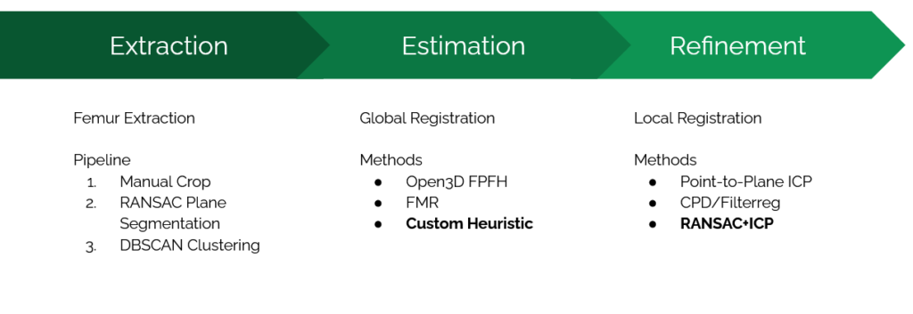
1. Extraction
Extraction involves filtering out noise and isolating a small region from the entire point cloud that contains the femur. This extracted point cloud is used for downstream registration algorithms. The steps include:
- Annotation:
The user annotates points on the femur and tibia. This approach is more reliable than heuristic methods or object detection models. - Segmentation:
Annotated points are used as input for segmentation, leveraging Meta’s Segment-Anything Model (SAM). Empirical observations showed that ICP registration performs best when only points from a single bone (e.g., femur) are present. This step produces a 2D mask of the bone, which is then unprojected to obtain a “masked” point cloud.
2. Estimation
Estimation refers to global registration, providing an initial estimate of the transform between the source and target point clouds before performing ICP. Key techniques include:
- Manual Alignment:
A custom heuristic assumes certain priors to align the point clouds effectively. - Depth and Angle Priors:
- Depth from the annotated femur point provides a precise position estimate.
- The angle between the annotated femur and tibia points gives an accurate yaw estimate.
These techniques result in an initial estimate very close to the ground truth, as depicted below in Figure 5:
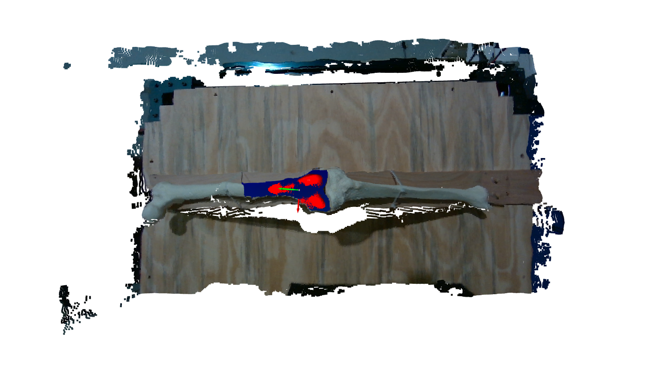
3. Refinement
Refinement involves local registration techniques such as ICP (Iterative Closest Point) for final alignment. While other methods like CPD/Filterreg were explored, vanilla ICP was ultimately selected due to its reliability. Enhancements include:
- RANSAC-like Trials:
Multiple ICP trials with random noise added to the starting position. However, this method was slow. - Directional-ICP:
A custom approach with predefined offsets for 10–12 trials, offering a faster and more consistent refinement process.
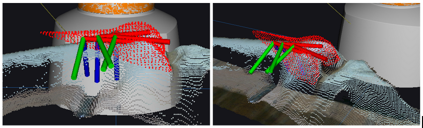
An example is shown below in Figure 6 of how we perform multiple trials of ICP to find the optimal alignment.
The final registration result is shown below in Figure 7.
The results are good enough to achieve an accuracy of less than 2 mm error for the overall system. Performance benchmarks (measured on a 4070Ti GPU) are as follows:
- Segmentation inference: ~40 ms (small SAM model).
- Unprojection and global registration: Negligible time.
- ICP trials: ~10 ms per trial, totaling ~100 ms for 10 trials.
- Overall time: ~300 ms for both bones.
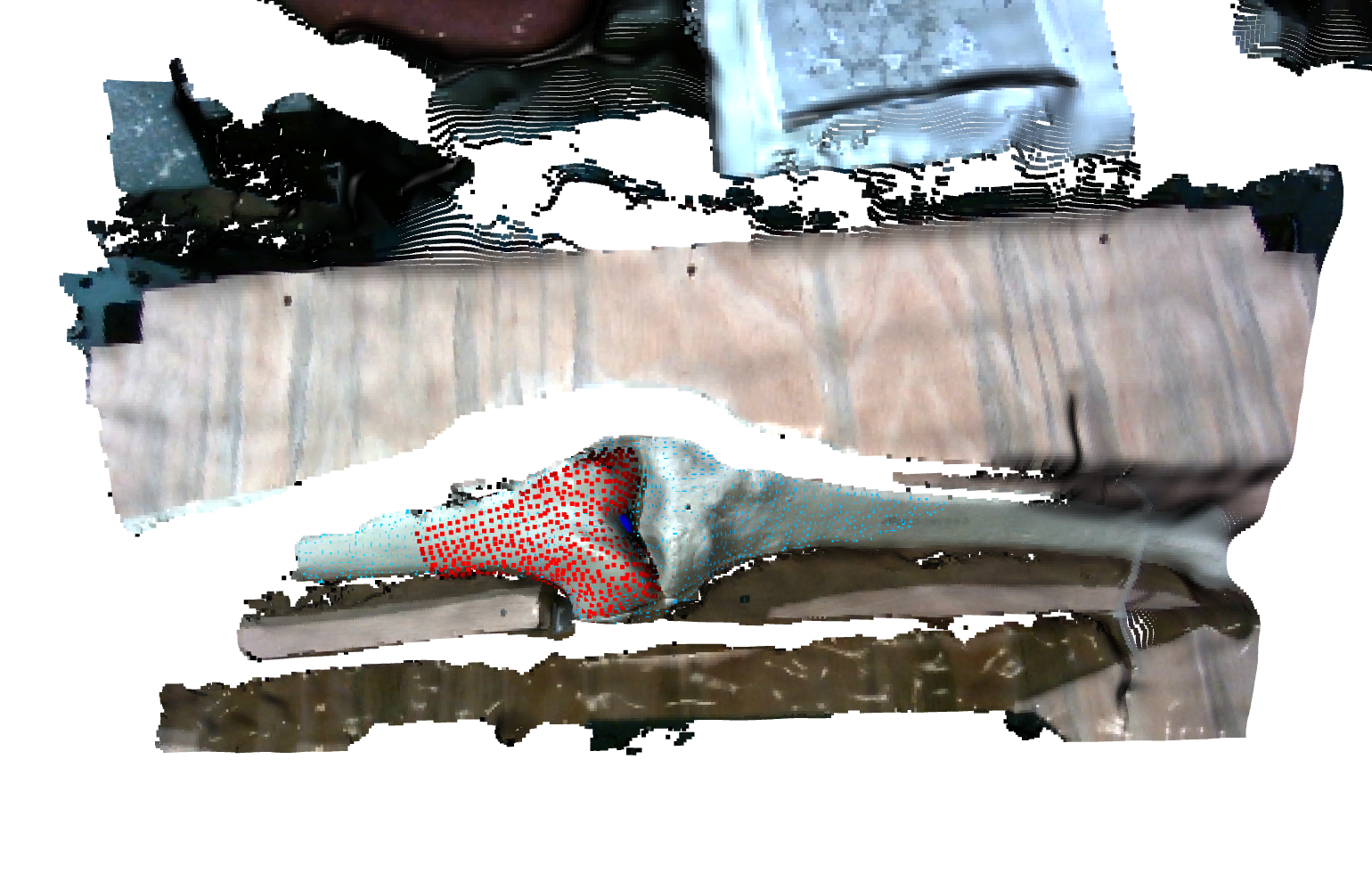
The entire process (excluding user annotation) is performed twice, once for each bone. The overall result with both femur and tibia registration is shown below in Figure 8.
The entire process of user annotation followed by registration on the live feed is shown below in a snippet from our FVD Encore demonstration in Figure 9.
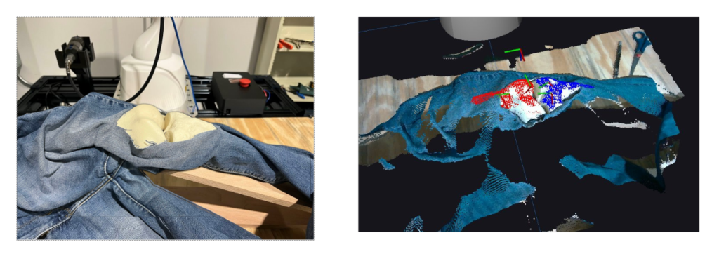
The overall pipeline is pretty robust and even works for scenes where the bone is highly occluded (which is the case in actual surgery). This is shown below in Figure 10.
Perception: Tracking
Since one of the major requirements is to compensate for motion, we need a dedicated Tracking module. To this end, instead of training a model from scratch, we decided to leverage the state-of-the-art any-point tracking model by Meta, called Co-Tracker. This model can track up to 70,000 points, although we only needed to track two points: the annotated femur and tibia points.
The key challenge was enabling the model to run on a live feed coming through a ROS topic. Although the model includes an online inference mode, it’s mainly designed to process video in chunks rather than frame-by-frame in real-time. To clarify how the model operates and its real-world performance:
- The way this model works is by keeping a buffer of 16 frames and running inference every 8 frames.
- Assuming the Realsense camera publishes at 30 FPS, that is waiting for 266 ms to get 8 new frames.
- Model inference time is 200 ms.
- Combining both these aspects, we can compute the effective performance of the tracking model to be 466 ms or 2.14 FPS.
This model is fairly robust and can even restore tracking after the object is moved out of the frame for a while. In addition to tracking estimates, it also gives a visibility value (boolean) for each point, which we use as a safety feature. We also compare the current position of the point with its previous position to mark the point as stable (if it is within a certain threshold). The tracking system is shown in action in the figure below:
The only caveat is that the model does place a heavy load on both the CPU and GPU and can slow down our registration pipeline.
We use the output from the tracking model in the following ways:
- Segmentation Assistance:
The segmentation model needs input points to segment accurately. We use the tracking model to propagate the initial user-annotated points so we can re-segment anytime. - Triggering Re-Registration:
Whenever the system is deemed stable, we inform the host node to trigger re-registration. This is only done once the system is stable, saving compute and only registering when necessary. - Hover Pose Generation:
Finally, we use the tracked point to generate a “hover pose” a few cm above the bone, which is given as the goal for the planning pipeline to monitor and compensate for motion safely.
Manipulation Subsystem
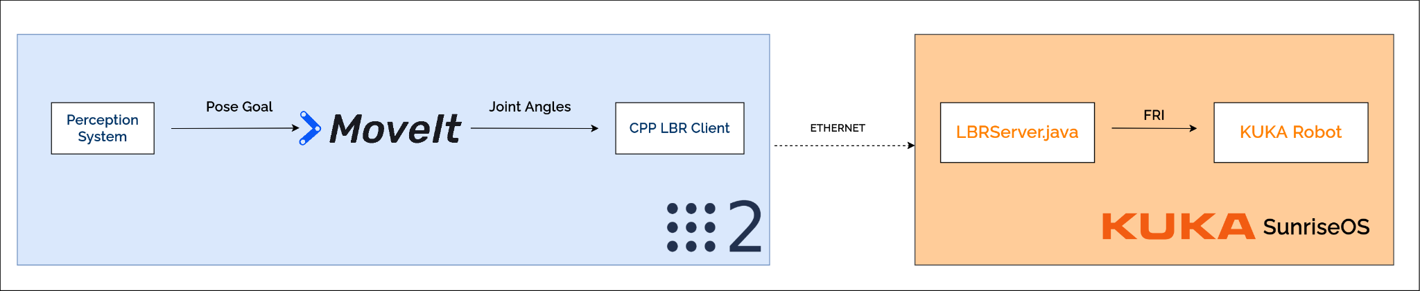
In SVD, our manipulation subsystem can only account for a static environment. Thus, one of the goals for the fall semester is to design and implement motion compensation. After some discussion, we decided to use the hybrid planning architecture to solve this problem. The architecture of hybrid planning is shown in Figure 12.
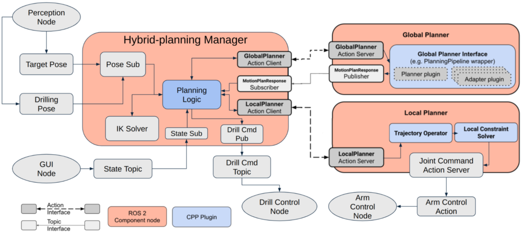
The architecture has three main components: the Hybrid Planning Manager (hereafter referred to as the Manager), the Global Planner, and the Local Planner.
- The Manager is in charge of taking planning goals, and it will delegate the planning problem to the Global Planner or the Local Planner according to the magnitude of bone motion. If the bone motion is large(Euclidean displacement > 7 cm), the Manager will request the Global Planner to plan a trajectory and wait for the trajectory response from the Global Planner. Once the response is received, the Manager will request the Local Planner to execute the trajectory. If it is a small bone motion (Euclidean displacement ≤ 7 cm), the Manager will request the Local Planner to go directly to the new pose. The Manager is equipped with the pick_ik inverse kinematics solver and can transform the target pose into a joint space goal. The Manager also employs one finite-state machine to switch between tracking and drilling motion. The state transition is automatic but can also be set through the GUI.
- The Global Planner utilizes MoveItCpp with Pilz Industrial Motion Planner. It can plan a long trajectory in Cartesian space. Since we assume there is no obstacle in the scene, we use the Pilz Industrial Motion Planner to decrease planning time and generate a more predictable path when compared to the RRT planner series.
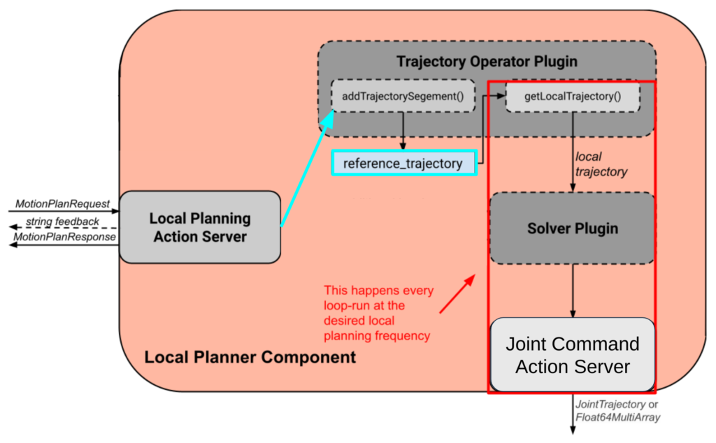
- The Local Planner holds a reference_trajectory at all times and is constantly running a loop at 10 Hz. Figure 13 shows the architecture inside the Local Planner. In every loop, the local planner takes a small chunk of the reference_trajectory and solves the control problem. After finding the solution, the Local Planner will output the control command to each joint on the KUKA arm. The Manager can modify the reference_trajectory through the action client talking to the action server. With the buffering reference_trajectory, we can achieve real-time motion compensation smoothly.
Input and Surgeon I/O
Input to the system consists primarily of two elements, and both of these are pre-computed and will not change during operation:
- Pre-Operative Bone Model is the STL file of the (femur/tibia) bone model we will attempt to register. This model can be exactly the same as our physical setup (in practice, obtained via the scan of the patient’s bone) or a generalized bone model (that of an average human). As agreed with our sponsor, we will start working with the specific bone model but hope to make our registration robust enough to even work with generalized bone models.
- Pre-Operative Surgical Plan is the plan that defines the position, orientation, and depth of each hole that needs to be drilled. This will be a text file that provides these coordinates with respect to the bone model STL file. Thus, if we successfully register the bone model, we know the drill goal in global coordinates. An example is shown in Figure 23 in the Spring semester Manipulation section.
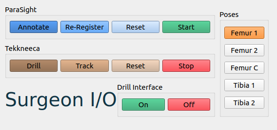
The surgeon I/O interface allows the operator to visualize the outputs of each module and send commands to the system based on the same. This system is written on top of RViz.
- Visualize the current status of the system: This includes live camera feed(s), the current position of the manipulator, the planned trajectory, and its progress along it.
- Send basic commands to the system: The UI functions to send data to the system, as seen in Figure 14 including software e-stop for the manipulator, software on/off the drill, and go home. The workflow is as follows:
- Annotate the femur and tibia. This is elaborated more in the perception section.
- Select which pose on the femur/tibia the system should drill.
- Enable tracking of the bones.
- Review the registration and either confirm it or re-register.
- If the registration is good, click the “drill” button.
- To stop the process midway, the “reset” button stops drilling and sends the robot home.
In addition, the operator can activate the emergency stop, which can cut off power to the system. Our manipulator already has an emergency stop, and we designed a separate emergency stop for our drill circuit as well.
Full System Integration
For the full result, please check out Component testing & experiment results.
Spring Semester
Hardware
Our hardware setup consists of the following:
- KUKA LBR Med 7
- Cameras – Realsense D405 / D435
- Vention Table
- Custom EE with Drill
- Bones with Bone Mount
- 3D-printed stencils for verification
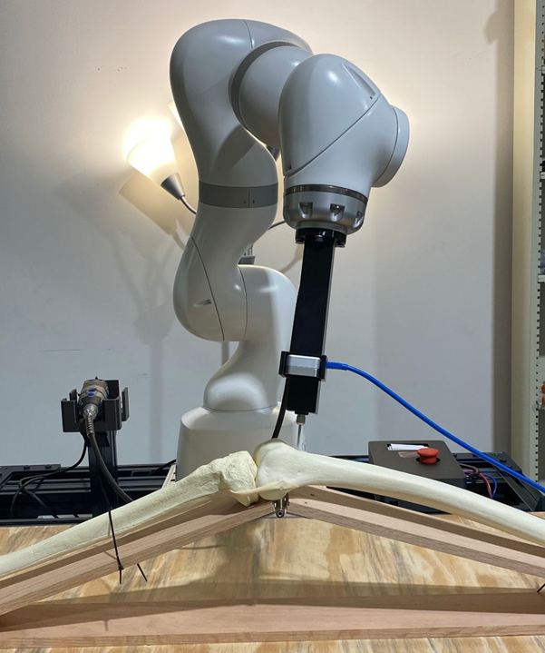
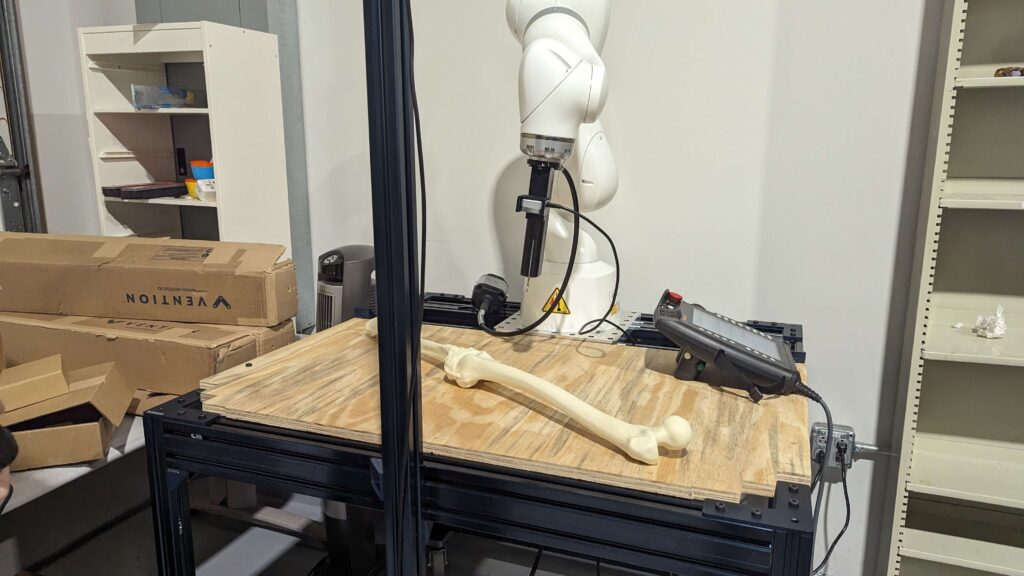
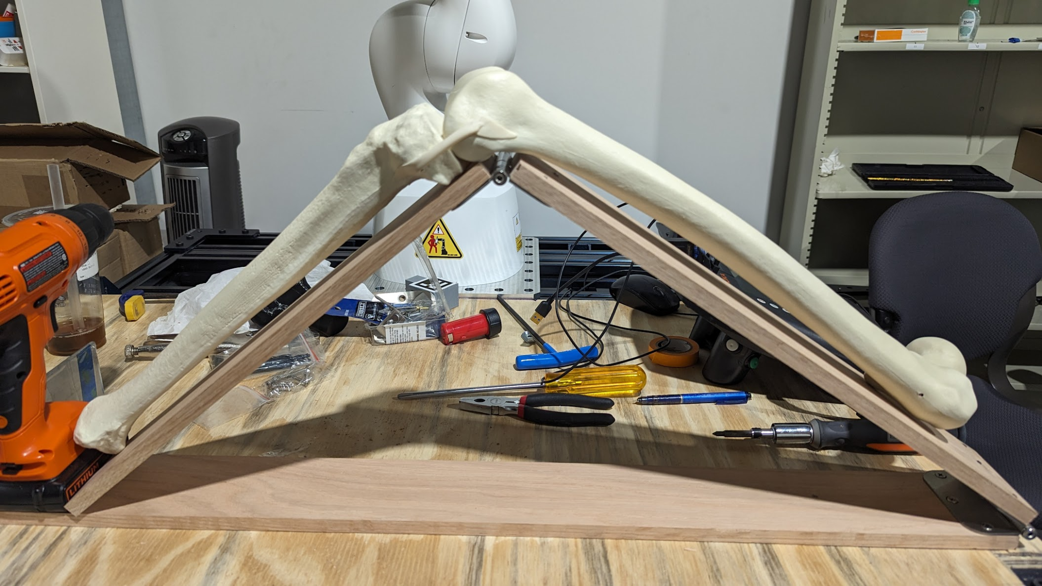
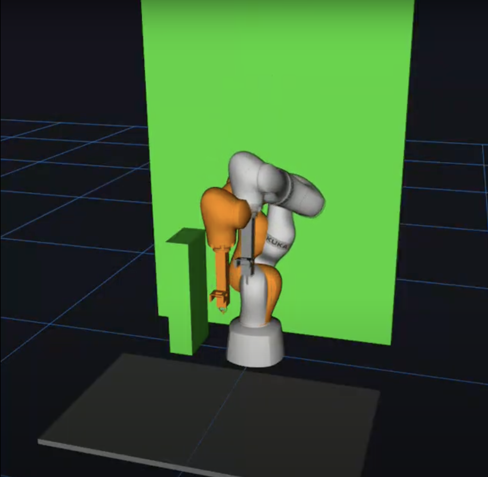
The overall setup is shown in Figure 1. Our sponsor, Smith+Nephew, provided us with the KUKA robot. We are also grateful to Prof. Oliver Kroemer, who generously provided a Vention table, which we later assembled.
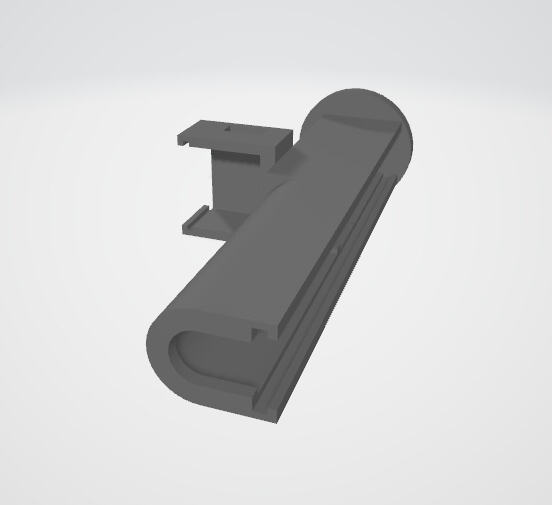
We designed a custom end-effector that can support both the Dremel 9100 drill and the D405 camera, which we later 3D-printed. The first iteration of our design is shown in Figure 2. We also built a bone mount that can hold the knee joint in flexion (Figure 3).
Drill Subsystem
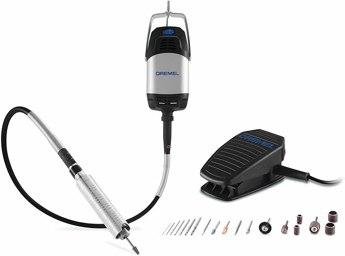
For the task of autonomous drilling, we have to interface a drill with our manipulator. After an extensive trade study between drills, we decided to select a Dremel 9100, as it met our desired torque, RPM, weight, and form factor. This Dremel comes with a foot pedal for actuation, which made us hypothesize that it would be relatively more straightforward to put a custom electronic actuation setup to replace the foot pedal (See Figure 4).
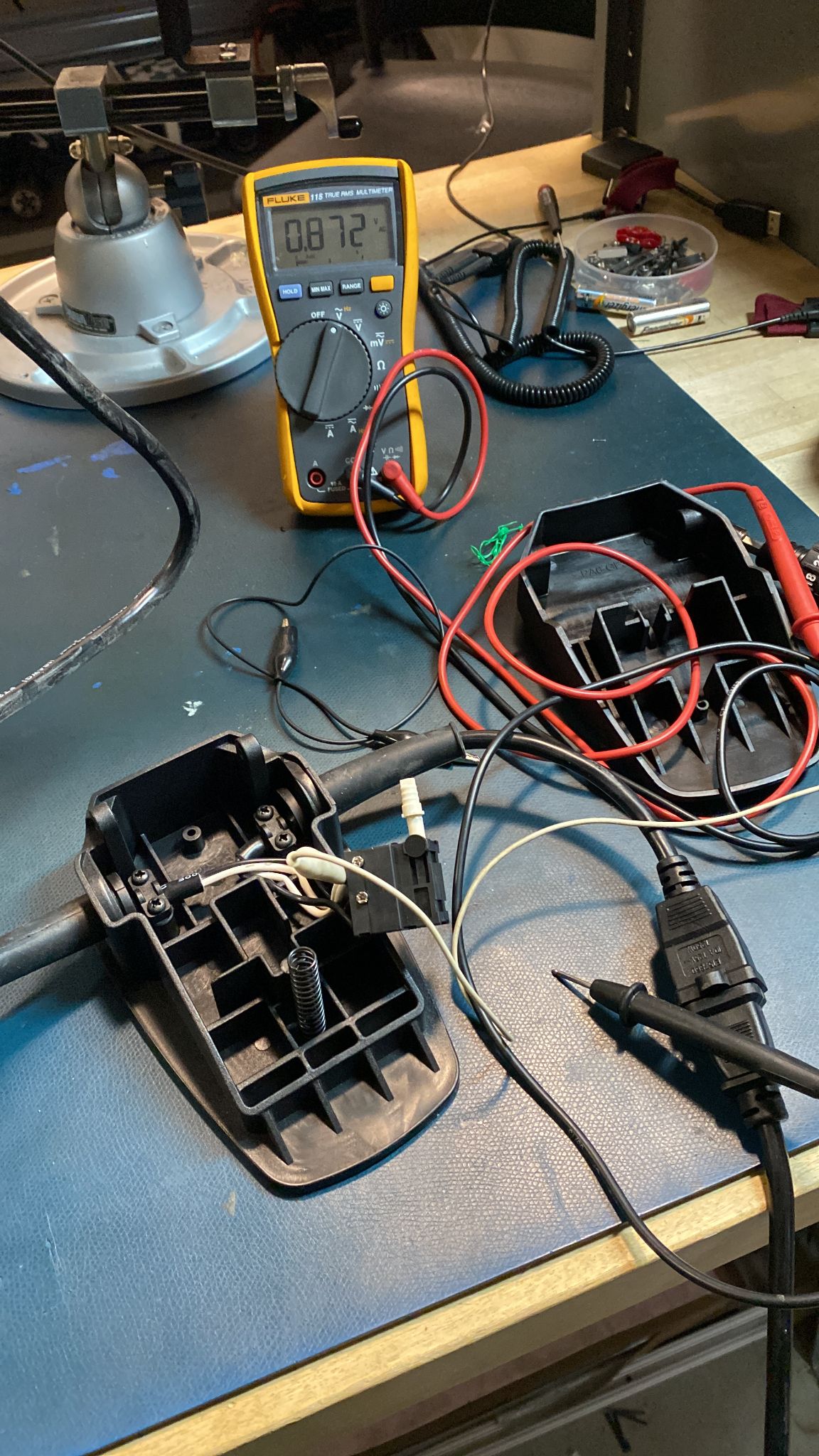
As seen in Figure 5, we examined the internal circuit of the foot pedal, and we realized it was operating like a potentiometer. In order to convert the spring compression to an electronic voltage, we decided to use a solid-state relay. For the input to the solid state relay, we used an Arduino UNO, which would provide a 5V digital high output when desired and 0V when we wanted to turn the drill off. The output from the solid state relay is AC Mains. The Arduino thus receives a “drill” or “stop” command over serial and converts that to a digital High or digital Low, respectively, on pin 13.
This serial command has been programmed to be sent by a ROS 2 node with PySerial, when the manipulator reaches the desired goal. Along with the solid state relay, we have added a dimmer switch potentiometer in the circuit, which allows the surgeon to manually control the speed of the drill, in case of emergency. This functionality is not pertinent to the autonomous nature of the drill.
To ensure the safety of our entire setup, we have added a bright red Normally Closed emergency stop to the mains of the circuit. Upon pressing this button, all power to the drill is immediately ceased.
This system was tested on multiple levels, first by writing to Arduino Serial, then with Python code writing to serial, thirdly with a user manually writing to the topic that the drill node subscribes to, and only after we were confident of safety and functionality, did we reach the fourth and final testing, where the manipulator autonomously actuates the drill.
Perception Subsystem
The primary task of the perception module is to perform registration to localize the bone in front of the robot so that we know where to drill. The idea is to collect a point cloud scene of the bone setup using the D405 camera and register the STL file we have of the bone to the scene. We started by using Open3D’s Point-to-Plane ICP to attempt registration but the results weren’t good enough. In Figure 6 below we show a sample point cloud we collected of a 3D-printed bone and our registration results.
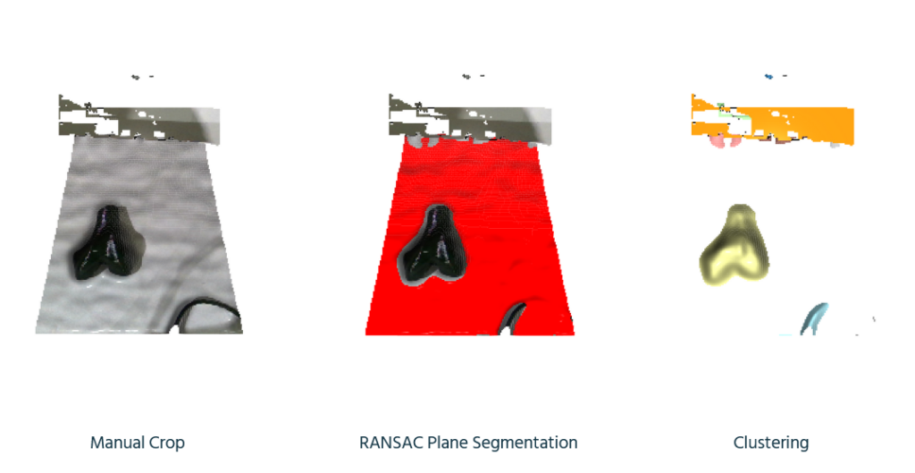
We later realized that it was because we were not properly processing and filtering the point cloud to remove noise. Thus we made a point cloud processing pipeline that uses techniques like RANSAC and clustering to just extract the bone area (Figure 7). The extracted bone point cloud is shown in Figure 8.
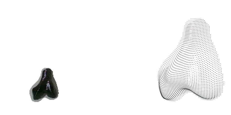
After extracting the bone area, we attempted ICP registration again but it didn’t give good enough results. So we decided to try a deep learning-based method called Feature Metric Registration which achieves much better alignment as shown in Figure 9.
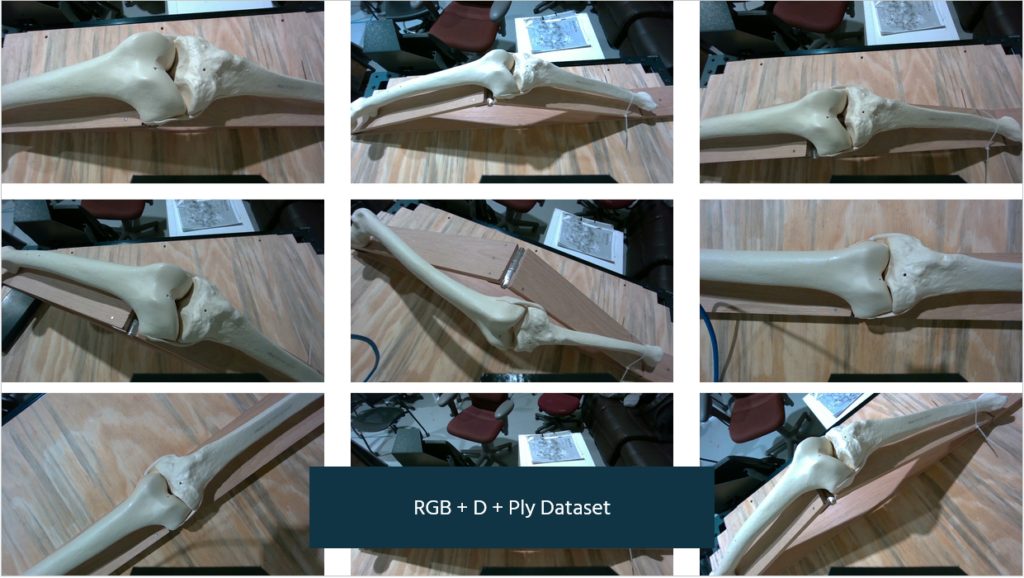
But this was just tested on a single random scene and may not be reflective of our actual data distribution. So we have collected a point cloud dataset using the end-effector armed with a D405 and the actual bone setup (Figure 10).
But as expected the above-mentioned algorithms didn’t work well on this data so we realized we need to take a more structured approach to this problem.
The overall registration pipeline consists of 3 stages as shown in Figure 11.
After exploring various methods we realized a custom heuristic works best for global registration where we manually align the centers of the two point clouds. We then perform ICP, but in a RANSAC fashion where we perform 100+ trials. In each trial, we first add Gaussian noise to the initial transformation we get from global registration (Figure 12).
Then we perform ICP for each trial and then return the transformation with the best fitness score across all trials. This results in a rather robust registration result that worked for 12/16 samples in our dataset. Results across different point clouds are shown in Figure 13 and the final overlaid result is shown in Figure 14.
We finally performed camera calibration and refactored the entire Open3D pipeline to a ROS2 package to integrate working with live realsense feed and the rest of our manipulation stack (Figure 15).
The overall pipeline is perfectly functional and has been integrated with our manipulation pipeline. This is what was used for our Spring Demonstrations and we were able to achieve <8mm error. But we assume certain priors for registration that limits the system’s ability to generalize to various scenarios –
- Femur is always on the left
- Femur is within the manual crop region
- Femur makes less than 45 deg angle with the horizontal axis
Thus we have been developing an alternate registration pipeline that tries to leverage state-of-the-art foundation models. This consists of a combined extraction plus global registration step as shown below in Figure 16.
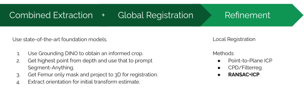
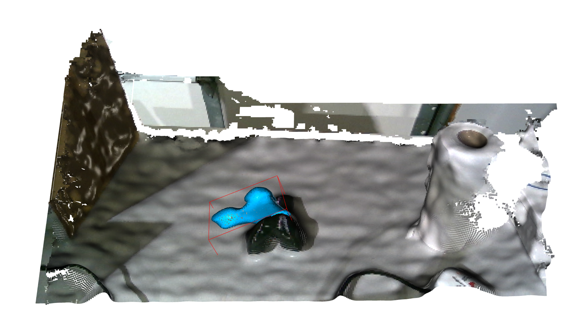
This consists of the following steps each of which are shown visually in Figure 17 –
- First we use GroundingDINO with the prompt “bone” to find an initial bounding box. This step effectively replaces the manual crop in the original pipeline with a more dynamic variant. We also tried the prompt “femur” but that still gives us the overall bone region instead of just the femur.
- Then we project the point cloud within to a depth image of the region and extract the point with minimum depth (since in flexion this will almost always lie on the femur).
- We then use Segment-Anything (SAM) to get a mask of just the femur region. SAM can either take a bounding box or a specific point as input but we can’t directly give it the DINO bounding box since that is of the whole bone. So we instead compute a point that is guaranteed to lie on the femur in the previous step which is given to SAM to obtain a femur mask.
- By fitting a
cv2.minRectusing OpenCV we are also able to extract the orientation (the red vector) which can be a good initial registration estimate.
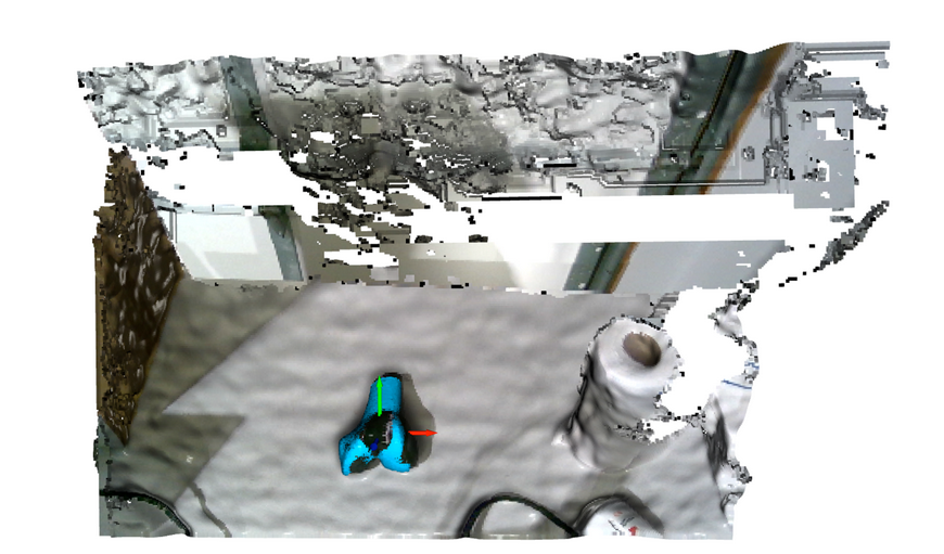
Finally we find points that lie within this mask (by using the camera instrinsics) and are thus able to find a target region that just consists of the femur. We then use RANSAC ICP as in the original pipeline to refine and obtain the final alignment. Results are shown in Figure 18.
For future work, we will incorporate the additional D435 top-down camera which will be used to track motion for dynamic compensation. This will also require us to improve the performance of our registration pipeline. Currently it takes a few seconds to register and we eventually want to be able to register multiple times within a second.
Manipulation Subsystem
For our manipulation stack, we intend to use MoveIt for motion planning. For this, we are using the ros2_lbr_fri package. We first set up the package in simulation with Gazebo (Figure 20) and synced it with our manipulator, enabling us to control the KUKA Arm with MoveIt. The overall architecture is shown in Figure 19.
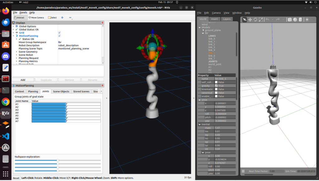
But the above example was controlled via the GUI, and we needed to control the arm programmatically, so we started working with MoveGroupInterface.
To plan for the Kuka arm, we need to write a MoveGroupInterface to communicate with the Kuka MoveGroup. Because our MoveGroup is launched under namespace /lbr, we also launched the MoveGroupInterface under the same namespace and remapped the action server/client to make MoveGroupInterface communicate with MoveGroup. With MoveGroupInterface, we can select the planner used for planning and can add static obstacles (motor mount, table, and virtual walls) into the planning stack (Figure 21). We later removed the static obstacles for the final integration for more predictable planning.
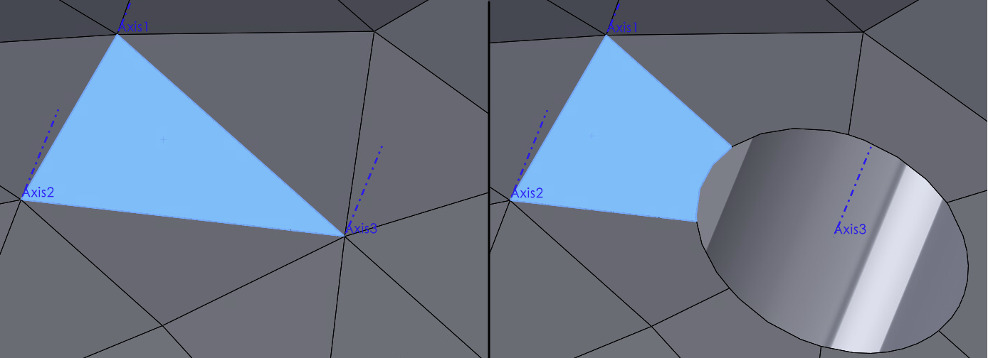
To make the drill reach the desired drilling pose, we first need to define the surgical plan. A surgical plan is a drilling point and a drilling vector. To define it on an STL file, we choose three points to form a face, so we can use the normal vector of the plane as our drilling vector, and a point on the face (selected the last point from three points in counter-clockwise order) to be the drilling point. With Solidworks (Figure 22), we can easily output the STL file and port it to Open3D (Figure 23).

Perception <-> Manipulation Integration
Finally, we take the pose provided by the perception system after registration and make the manipulator move to that pose (Figure 24).
We also execute this on the actual robot. Originally, there was some calibration error, so the manipulator didn’t quite reach the desired goal (See Figure 25).
However, after refining the registration pipeline and re-calibrating the extrinsic matrix, we get better accuracy, as shown in Figure 26.
Full System Integration
We put all the systems together and measured the final drilling accuracy to evaluate our system. Our target criteria is to be within 8mm of the desired goal. In practice, we observe that our system is always within 8mm and, more often than not, within 4mm. The final drilling results are shown in Figure 27. For the full result, please check out Component testing & experiment results.