Emergency braking for obstacle avoidance

DJI provides Onboard SDK which can be used to communicate with DJI flight controller to receive real-time data and to control the quadcopter. Our DJI interface is built around the ros wrapper of Onboard SDK which allows receiving data as ros topics and publish commands by subscribing to ROS services.

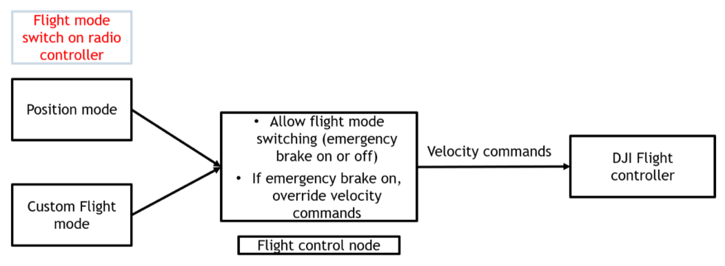
DJI provides information related to state of the aircraft which includes position, attitude, velocity, pilot commands, etc. A separate node was written for emergency brake functionality. This node subscribes to pilot control inputs and based on position of a switch on the radio controller it either enables or disables our custom flight mode. This custom flight mode converts pilot commands to velocity commands for the quadcopter. These velocity commands are constrained if pilot’s commands are leading to a collision. 

For obstacle avoidance we can easily determine the time to impact from zeroing the speed equation and introducing its value back into the position equation.

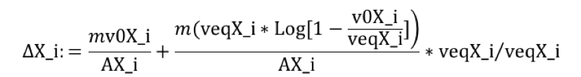
This equation can be solved for the equilibrium speed that a pilot input should give, that given a non-zero initial speed at a particular point, would stop at the obstacle location. Nonetheless, the equation is transcendent (product log) and Matlab/Mathematica are really bad solving it (C++ is bound to be even worse).

Instead of doing this, we solve for two types of situations that are really simple: the “No Return” range (what is the distance the quad travels starting from a non-zero speed and having full reverse input) and the “Zero Input” range (the distance the quad travels with a zero input when starting from a non-zero initial speed).

We then fit a straight line between the two limit cases, simplifying the inverse dynamics and getting a control that reacts faster than the original function and should be more stable than a non-linear control with a function whose numerical computation is problematic. As a bonus, the straight line can be extended beyond the “Zero Input” as we no longer have a domain problem as we did in the “Product Log”. The point where we can give maximum input in the direction of the obstacle and still stop on time is referred to as “Full Control”.

With this approach we were able to operate seamlessly in four different regimes:

• Type I: The quad is in a state where the obstacle is further away from the “Full Control” and the pilot can do whatever he pleases
• Type II: the quad is in a state where the obstacle is further than the “Zero Input” range and the algorithm operates in the region of positive thrust inputs (which is a one to mapping to a target steady state speed) that tend gradually to zero as the obstacle approaches
• Type III: the quad is in state further away from the “No return range and the algorithms operates in the region of negative thrust inputs that tend gradually to zero as the object approaches
• Type IV: the quad is in a state closer than the “No return” range and only accepts inputs of “full reverse”

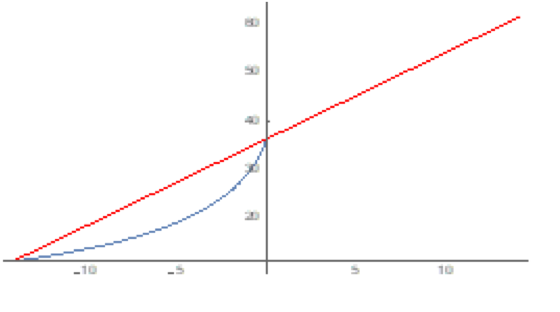
So, in directions where there are no obstacles, the pilot is by default in the “Type 1” regime. The detailed test cases can be found in the Annex 1 of this report. In figure 11:

• Y is the computed range (output in m), X is the equilibrium speed (input in m/s)
• Blue is the “real” product log function and

Red is the simplified control (please note that this is not a classic linearization about a single point instead it is a simplification that fits across two different points/regimes).