System Implementation

Overall System Depiction

The CraterGrader worksystem is comprised of a mobile robot and the supporting infrastructure set up around the platform. Images of the integrated vehicle can be seen in Figure 1. The full system is broken into ten distinct subsystems, displayed below in Table 1. At a high level, all subsystems are built around the Rover subsystem which acts as the mechanical and electrical hub for all development.

N	Subsystem Name	Functional Description
1	Sensing	Sensors, Sensing Nodes, Drivers, Filtering
2	Localization	EKF and Independent Localization Nodes
3	Perception and Mapping	Perceptive Filtering, Mapping, and Map Services
4	Planning	Low, Mid and High Level Planners
5	Controls	Motion Control and Mid Level Control & Odometry
6	External Infrastructure	Site Infrastructure, Networking, Test Site, Sensing
7	Rover	Mobile Platform Hardware, Electrical and Mechanical
8	Tools	Actuated Blade and Dragmat
9	Compute	Xavier and Arduino Companion Computer
10	Verification and Validation	Sensing, Software and Methods for Precise Terrain Measurement, Metric Tracking

Sensing Subsystem

The sensing subsystem consists of a variety of sensors for the purposes of localization as well as perception. A VectorNav VN-100 AHRS mounted to the chassis measures 3-axis linear acceleration and angular velocity. The VN-100 runs an onboard EKF to generate roll and pitch angle estimates by fusing the accelerometer and gyroscope data. Although this sensor is capable of computing a yaw angle estimate as well by fusion with magnetometer data, this information is omitted for the purposes of this project to better mimic the constraints of operating in a lunar-like environment. 

Operating on the moon presents additional challenges in sensing, such as working in a GPS-lacking environment. In the absence of GPS, the system uses a robotic total station, mounted external to the worksite, in conjunction with a reflector placed at the top of the vehicle, to compute an absolute position estimate via time-of-flight signaling. Figure 6 shows an example of the robotic total station.

A fiducial-tracking fisheye lens camera is used to compute an absolute bearing estimate with reference to AprilTags placed around the worksite. AprilTags are used to emulate the behavior of a sun-tracking sensor in the indoor test environment. On the lunar surface, a similar sensing modality could be used to compute absolute heading with respect to the sun.

An Intel RealSense D435i camera is mounted on the sensing mast of the vehicle and is used as the primary sensor for terrain detection. This stereo vision camera publishes point cloud information that can be used to identify terrain topography. Figure 3 depicts sample point cloud data of a crater in the worksite as received from the RealSense, alongside the equivalent reference terrain. The full list of sensors with part numbers and quantities are displayed below in Table 2.

N	Sensor Name	Measurement	Type	QTY
1	Leica TS16	[x y z]	Robotic Total Station	1
2	RealSense D435i	[terrain distances]	RGB-D Camera	1
3	‎‎ELP LYSB01N03L68J	[yaw]	RGB Camera “Sun Sensor”	1
4	VectorNav VN-100	[roll pitch] [acceleration x y z]	AHRS	1
5	NE12	[quadrature counts]	Encoder	5

Localization Subsystem

The localization subsystem fuses IMU readings, total station data, relative pose from the AprilTags, and encoder telemetry to estimate the 3D pose (position and rotation) of the robot. The implementation leverages the ROS2 package robot_localization, which fuses data from the sensor suite via an Extended Kalman Filter (EKF). In order to have access to continuous motion as well as accurate global position, two EKFs are run in parallel: one representing the robot’s position in the relative ‘odom’ frame, which drifts over time, and the other in the global ‘map’ frame, which can have discontinuous updates to the position in order to correct for pose estimation drift. The graphical localization architecture is illustrated below in Figure 4.

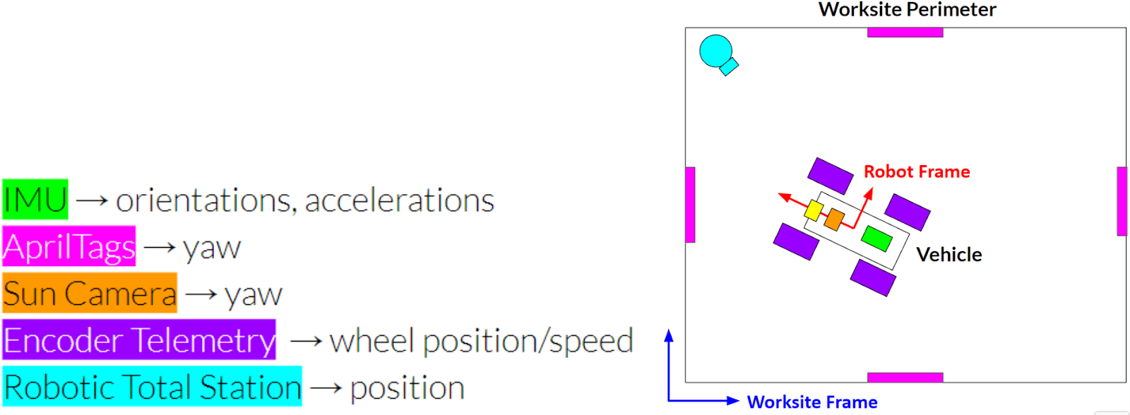
The localization subsystem provides an accurate and precise estimate of 3D pose. The total station provides a highly accurate 3D position estimate and the IMU provides 3D orientation and acceleration (excluding yaw). The yaw estimation procedure in Figure 6 outlines how noise in both the AprilTag orientation and distance are avoided, and only the precise directional axis from the camera to the tag is used. The axis is combined with the highly accurate total station position for accurate yaw estimates by computing the yaw from the position and an angular offset from the axis, roll, and pitch. The pose estimate is fused with the encoder telemetry in the EKF, empirically tuned in the sandbox, to estimate the most likely continuous pose of the robot. Although not used within the planning, slip estimates can be obtained by comparing the velocities in the odom and map frames, which could be used to improve planning and controls.

Perception & Mapping Subsystem

The Perception and Mapping subsystem takes raw data from the sensing subsystem and fuses it with a filter-based mapping approach to understand the terrain in the worksite. This system effectively transforms each point obtained by the stereo camera into the map frame and then bins each point into a map grid cell, with box filter rejection of points that lay outside the worksite. As points are binned into the map, the information is fused by modeling each map cell as a 1D Kalman Filter. The filter approach to mapping allows for different confidence estimates of incoming points based on any hand crafted noise estimates, or could allow for noise injection into the map based on robot disturbance of grid cells. Figure 7 depicts the resulting 2.5D grid map representing various binned heights at grid cell locations that have been seen by the robot. 

Planning Subsystem

The planning subsystem is responsible for generating a high-level plan for coupled mobility of the robot platform and grading blade. This plan is computed given the state of the robot and its environment, to fulfill the robot’s overall objective of leveling worksite terrain.

Behavior Executive

At the heart of the planning subsystem is the Behavior Executive which ties together the system concept of operations with the subsystem architecture. The Behavior Executive is primarily responsible for interfacing to subsystem modules to manage the planning subsystem for driving the system actions. Secondary responsibilities include monitoring system health and fault handling. 

Functionally, the Behavior Executive connects the Planning subsystem to Mapping data products in order to compute worksystem trajectories and then send those trajectories to the Controls subsystem for real system motion. Additional checks include monitoring the trajectory following process in order to determine if and when new trajectories are computed. Accounting for vehicle slip to enact fallback/escape maneuvers in case the system got stuck was explored but ultimately deprioritized for development as embedding was observed to have very low probability of occurring. 

The Behavior Executive is implemented as a hierarchical finite state machine with two levels of states; Level 0 and Level 1. A C++ class structure as depicted in Appendix B is adopted in order to safely allow states access to machine parameters and trigger transitions. Level 0 contains the lowest level states that carry out actual computation and system behavior calculations. Level 0 includes states for updating the map, running the transport and kinematic planners (explained below), and following the computed trajectory. Figure 8 depicts these states with their transition dynamics. Note that states related to escape maneuvers and fallback handling were not fully implemented. Level 1 distinguishes between Exploration and Transport phases of system operation to drive Level 0 behavior. All Level 0 states are impacted differently by these two phases as described in Table 3.

State (L0 or L1)	Exploration_L1	Transport_L1
UpdateMap_L0 (Both Exploration & Transport)	Only when the map is updated, it puts the FSM into a state to check if the sitework has been completed based on the updated map in its new state (SiteWorkDone_L0).
SiteWorkDone_L0 (Both Exploration & Transport)	End mission (EndMission_L0) if the current measured map is within design thresholds of the target design map, otherwise it goes to check if the map has been explored or not (MapExplored_L0).
MapExplored_L0	On the first pass, it will plan the exploration (PlanExploration_L0),	Every other time, it will replan the transport (ReplanTransport_L0).
PlanExploration_L0	Attempts to plan the exploration, when it succeeds, it will attempt to get a set of goal poses from the exploration plan (GetExplorationGoals_L0).	N/A
GetExplorationGoals_L0	Gets all the exploration goal poses and puts the robot in driving mode towards these goals (GoalsRemaining_L0).	N/A
ReplanTransport_L0	N/A	Plans the transport plan once at the start (PlanTransport_L0), only replanning if map state has been updated every N number of times, currently set to never update and only get the previously planned goals (GetTransportGoals_L0).
PlanTransport_L0	N/A	Computes transport plan using Earth mover’s distance optimization, resulting in a set of goals that is accessed (GetTransportGoals_L0) for motion planning.
GetTransportGoals_L0	N/A	Gets all the transport goal poses and puts the robot in driving mode towards these goals (GoalsRemaining_L0).
GetWorksystemTrajectory_L0	Calculate the exploration trajectory using the kinematic planner that includes the velocity targets but with no topography cost. If the trajectory was successfully calculated, the worksystem is enabled and begins to follow the trajectory (FollowingTrajectory_L0).	Calculate the transport trajectory using the kinematic planner that includes both the velocity and tool targets, and also considers the topography cost. If the trajectory was successfully calculated, the worksystem is enabled and begins to follow the trajectory (FollowingTrajectory_L0).
FollowingTrajectory_L0 (Both Exploration & Transport)	Until the goal is reached, the robot will use its control system and follow path, velocity, and tool targets. Either the worksystem fails to reach the goal pose due to sufficient accumulated error from trajectory, requiring a trajectory replan (GetWorksystemTrajectory_L0), or it reaches the goal and seeks the next goal pose (GoalsRemaining_L0).
GoalsRemaining_L04 (Both Exploration & Transport)	If there are goals left, obtain the next one and go to calculating the trajectory (GetWorksystemTrajectory_L0). Otherwise, the work system checks if the map has been updated (UpdateMap_L0).
EndMission_L0 (Both Exploration & Transport)	All processes stop as the worksystem has completed its mission objective of matching the measured map with the target design map topography.

Exploration Planner

The Exploration Planner is responsible for providing a feasible set of waypoints to encourage full worksite traversal during the Exploration phase. In practice, this is accomplished by placing waypoints along a ¾ circumference circular arc to map out the worksite boundaries, followed by a three point turn which allows the robot to face the center of the worksite and map the remaining unseen areas in the middle. This general strategy was developed through manual driving trials to accomplish full worksite exploration in a kinematically feasible manner, and is depicted in Figure 9. Exact locations of the waypoints are parameterized by worksite dimensions, such that the radius of the circular arc and placement of other waypoints scale according to the height and width of the worksite.

Transport Planner

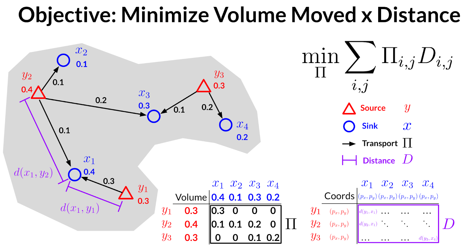
The Transport Planner solves a mixed integer linear optimization problem for minimal-energy terrain manipulation to convert an original map topography to a design map topography. The resulting solution is a set of transport assignments indicating which terrain volumes should be moved where. The solution is agnostic to manipulation modality so the plan can be extended to a variety of machine tools, such as both grading and excavation. The physical action of exactly how the terrain is modified is then left to a lower level kinematic planner that considers platform constraints. For example, in a grading application, the assignments become waypoint poses for the system to drive the grading blade to. To guide feasible driving trajectories with constrained turning radius, an additional waypoint was placed rearward of the crater rim (source) waypoint. This results in triplets of poses that when traversed in order drive the system to move in and out of the crater to flatten the rim.

The planner uses nodes defined with a certain amount of volume and planar coordinates within a worksite as shown in Figure 10. A set of “source” nodes are the position of volumes that are above the design topography and a set of “sink” nodes are the position of volumes that are below the design topography. The planner adopts concepts of volume in a distribution and distance moved between distributions from the Earth Mover’s Distance[], more generally known as the Wasserstein metric[], to solve for a plan of how much volume to move from each source node to each sink node while minimizing the total sum of volume moved multiplied by the distances traveled; analogous to mechanical work, ignoring transport rate. The transport matrix Π and distance matrix D are both n m matrices for n source nodes and m sink nodes. Constraints were made on the allowed volume moved from and to the source and sink nodes, respectively, as a binary mixed integer problem to account for the two cases of having more source volume than sink volume and vice versa. These constraints make the planner more robust to terrain variations and/or mapping inaccuracies to prevent online infeasibilities. The definition of these constraints, along with the full optimization problem description, are included in Appendix A. This planner was then implemented in C++ using Google OR-Tools [link] as a linear solver.

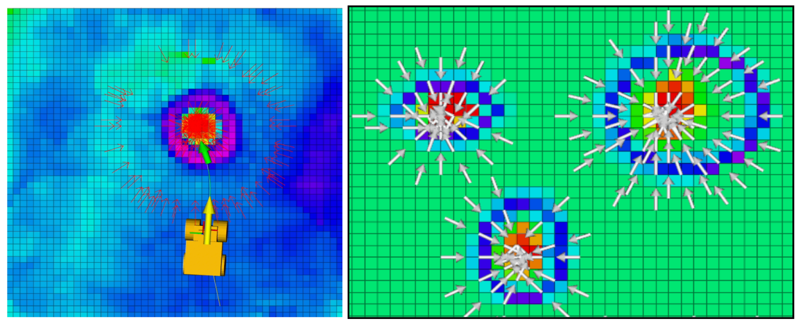
The result of the transport planner is run on the system in real-time after the map exploration phase is complete. For nominal operation with this work, the planner was run once prior to crater manipulation because localization and mapping had minimal drift and so did not require replanning. The system developed in this work was tested primarily on a single crater for the purposes of managing design and development scope, but the Transport Planner also seamlessly extends to multiple craters. Because this work focused on grading craters, the final transport plan assignments were filtered to only consider transport distance below a threshold, precluding worksite-wide manipulations, and spatially decimated because the grading blade on the system could effectively manipulate more than one node cell in one pass. Examples of transport plans for craters are shown in Figure 11.

The Transport Planner also works with arbitrary final design topographies. As an example for a lunar application, a design topography could be a flat landing pad with raised berms around the pad for blast ejecta shielding (Figure 12 & 13). The transport planner then calculates both how to modify terrain in order to form the new terrain structure, in this case berms, as well as remove unwanted structures, in this case craters. The plan still minimizes the total cost of how far the volumes are moved, and also considers overlapping and arbitrary features. Note that the grading system would not be able to dig effectively, so additional excavation tooling/machinery would be needed for this example.

Kinematic Planner

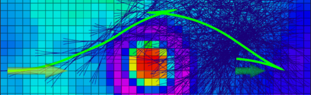
The kinematic planner comprises the lattice generator and A* search for XY path planning alongside the tool and velocity planner. The lattice generator creates a lattice relative to a specified position (beginning from the robot’s current position), both in front and behind the robot, to create a graph that is kinematically feasible based on the robot’s kinematic model. This graph is searched using A* and lattice are generated and appended to potential paths as the graph is being searched in order to find a path towards the goal pose. The A* is weighted and accounts for the topography cost and distance when searching for the optimal path. The topography cost minimizes the likelihood of climbing heights, as shown in Figure 14, which helps lower the likelihood of getting stuck. 

Once an optimal path is found by the A* search, a velocity planner assigns a target velocity to each waypoint along the path. This target velocity is simply a fixed positive or negative value depending on whether the robot is intended to travel forward or backward  respectively at a given waypoint. 

Finally, the tool planner assigns a target blade height to each waypoint. The blade height is determined by a simple heuristic, coined AutoGrader, and lowers the blade to a empirically tested design height when the robot is driving forward during the transport phase, and raises the blade when backing up to avoid unintentional dragging of material or unnecessary drag forces when backing away. Although simple, this heuristic is highly effective due to the architecture of the transport plan that aligns poses for pushing highs into lows within the worksite to reach the target design topography.

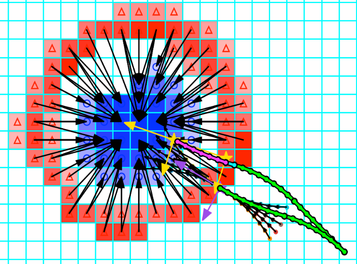
When combined with the transport planner poses, the Kinematic Planner guides the worksystem to drive in and out of the crater in a normal direction while tangentially traversing the rim. An example set of trajectories for navigating to the rim, pushing terrain in, and then reversing out is shown in Figure 15.

Controls Subsystem

The controls in this worksystem can be decomposed into two separate levels: the worksystem controls and the actuation controls. Worksystem control considers the current trajectory and robot state, and provides position and velocity actuator commands to best minimize robot state errors based on methods described in the following sections. Actuation control takes these commands and acts as the lowest level control layer of the autonomy stack, interfacing directly with the motor controller boards to minimize error in desired actuator command and actuator state.

Worksystem Control

Fundamentally, the worksystem control node is responsible for computing appropriate actuator commands for three distinct objectives: steering, driving, and tool motion. These objectives are decoupled for simplicity and are each assigned their own controllers, described in more detail below.The steering controller generates a single steer angle command applied symmetrically to the front and rear axles, with an architecture diagram shown in Figure 16. For a given reference trajectory provided by the kinematic planner, the “reference point” is identified as the closest point on the reference trajectory to the robot’s current position. Next, two error values are computed: the cross-track error, which is the lateral distance between the robot’s current position and a tangent line at the reference point, and the heading error, which is the delta between the robot’s current heading and the desired heading at the reference point. The steering controller uses a modified Stanley control law to determine a steer angle that aims to reduce or trade off these two error metrics. Figure 17 depicts the original Stanley control law compared with our modified version (where delta = steer angle command, e_h = heading error, e_c = cross-track error, k_h and k_c are tunable gains on corresponding error terms, v = longitudinal velocity, and k_s is a small softening constant to avoid division by zero). The key modifications made are: (1) the removal of the velocity term and softening constant in the denominator, as the robot tends to travel at low speeds which in practice would cause the cross-track error term to quickly saturate, and (2) the addition of a scalar factor applied to the heading error to further tune relative importance of heading versus cross-track error. An additional temporal moving average filter is applied to the steering command to further smooth the control signal, which is then sent to the motion control system (MCS) to control the steer actuators.

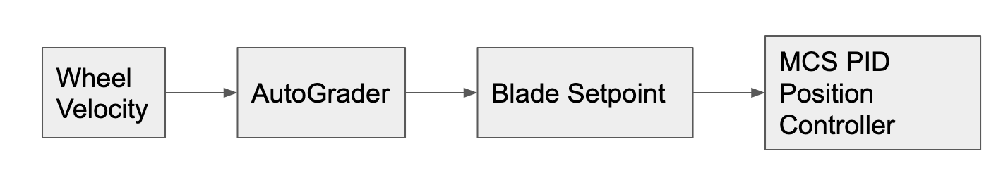
The tool controller uses the simple heuristic called AutoGrader (as described in Section 7.1.2.4.4) for giving a setpoint to lower level control. This heuristic was demonstrated successfully during SVD and FVD. The architecture is depicted in Figure 18.

Actuation Control

The actuation control subsystem is a standalone power and control subsystem, responsible for commanding motion to the actuators and relaying actuator feedback back to the main compute. There are five motors in total: one for driving and one for steering on each axle, and one for blade height actuation. Each of the motors features encoders to measure the angular position of our actuated components. This includes wheel encoders, steering encoders as well as an encoder to measure the height of our grading blade. Three RoboClaw motor controllers interface with the motors for the drive, steer, and tool control respectively, and utilize PID controllers to control each motor with reference to either an actuator position or velocity setpoint coming from worksystem control.  An Arduino Due running micro-ROS is used to bridge the ROS2 stack running on the Xavier to the low-level motor controllers. Figure 19 illustrates the architecture of the motion control subsystem, including the power source and distribution system along with the electronics and actuators.

External Infrastructure

The project utilizes the large purpose built “Moon Yard” in the Planetary Robotics Lab. The sandbox which was built in part by the team is approximately 600 sq ft and contains ample room for lunar excavation testing. This sandbox itself is considered the foundation of the external infrastructure, with some additional objects built upon it. One highly critical aspect of this infrastructure is the local network setup around the sandbox. This LAN allows the robot to communicate with the robotic total station by way of a TX2 built into an electronics enclosure shown below in Figure 20. The LAN also allows for human operators sitting at an operations terminal to send commands to start and stop the robot while receiving continuous information. AprilTags were placed around the worksite to act as the sudo-sun for yaw tracking.

Rover Subsystem

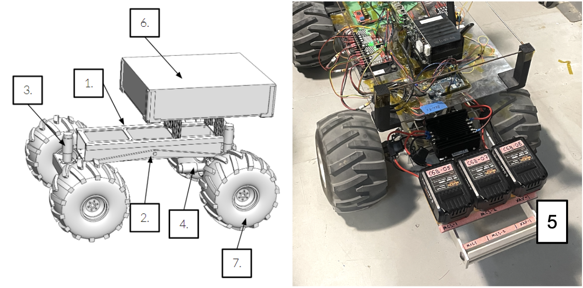
The rover subsystem includes all structural and mobility hardware that interfaces actuators, sensors, and compute. It is composed of the following (labeled in Figure 21) :

1. Chassis: 6061 modified square tube 
2. Suspension Assembly: Roll-averaging rocker
3. Steer Assemblies: Double-Ackermann
4. Drive Assemblies: 4WD, Front/rear Differentials
5. Battery System: 3x 20v 5.0Ah li-ion batteries with regulation and fusing (not pictured)
6. Electronics Box: Dust protection softgoods, polycarbonate substrate 
7. Wheels: Polymer exterior, foam core, high traction

Tools Subsystem

The tools subsystem is composed of mechanisms performing two modalities of earthmoving: grading and smoothing. The grading modality is achieved by a vertically actuated flat blade with statically adjustable yaw and pitch, shown in Figure 22. The smoothing modality is achieved through the use of a chainmail dragmat, shown in Figure 22, which removes high-frequency surface imperfections behind the vehicle.

The blade mechanism mounted to the center of the vehicle moves vertically with one degree of freedom and cannot be pivoted with roll, yaw or pitch due to previous testing and iterations where it was determined to be inconsequential for our dozing-like applications. A limit switch homes the blade position after power cycles and limits motion past the top of travel if control is lost. The dragmat is designed to be force limiting through its low stiffness plastic mounting bar. The dragmat has not changed in design since the initial concept before SVD.

Compute Subsystem

The compute subsystem consists of an NVIDIA Jetson AGX Xavier Development Kit running Ubuntu 18.04. The Xavier acts as a hub for computation to run the autonomy stack and integrates all external electrical components. A PCIe card is mounted into the connector pins as well, which provides 4 additional USB ports for our sensors that provide a dedicated 5 GBps line for each port. All software is run in a custom Docker container, set up for use with ROS2 Galactic with networking capability for a wireless ROS2 communications. A local network router in the MoonYard facilitates wireless ROS2 communications between the Xavier and an Nvidia TX2. The Nvidia TX2 compute connected to the same local network acts as the interface between the robotic total station and the vehicle compute, and additionally runs visualization to minimize onboard compute where possible.

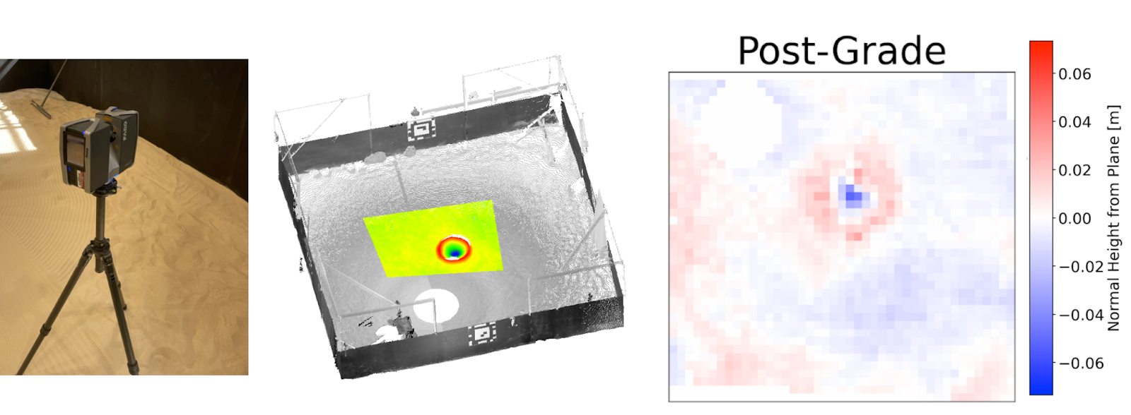
Verification & Validation

The purpose of the verification and validation (V&V) subsystem is to validate our robot’s performance post-operation, and to determine whether the system meets the requirements. A FARO Focus 3D laser scanner, as shown in Figure 23, is used to generate worksite scans before and after grading. An example scan is shown in Figure 23. After some subtle post processing in the open source desktop software CloudCompare, these scans are imported into our validation scripts, written in Python, which compute performance metrics such as surface grade and smoothness.