Detection

Implementation Details

Background Subtraction

The steps to achieve background subtraction with static LiDAR setup are listed below:

1. Load the pre-recorded background point cloud which contains a static environment without moving objects.
2. Within a callback function, initialize octree object.
3. Add background points into octree.
4. Switch octree buffer to receive new point cloud later.
5. Add current frame points into octree.
6. Execute comparing algorithm which extracts vector of points indices from octree voxels that did not exist in previous buffer.
7. Add and format the resulting points; publish the result via certain ROS topic.

One thing to note that I used a pre-recorded background point cloud as a reference. In the future, it should be dynamically generated by monitoring the real environment and taking consecutive frames of data.

Octree is an efficient data structure to store point cloud. The reason why I use octree to store the information is that by manually adjusting octree’s resolution, we can find similar-position points between background and current frame. As shown below, it achieves satisfying result even though LiDAR point cloud is effected by noises.

Euclidean Clustering & Centroid Computation

The steps to implement Euclidean Clustering with LiDAR point cloud are described below:

1. Load point cloud after background subtraction.
2. Duplicate the point cloud and modify all points to the same height.
3. Set Euclidean tolerance, minimum and maximum clustering size.
4. Perform the Euclidean clustering operation (Exhaustively and recursively search
   neighboring points within tolerance; save clusters fitting min/max threshold).
5. Iterate every founded cluster, compute the 2D centroid of all the points within that
   cluster (since heights are fixed in step 2).
6. Publish both clusters and centroids information to certain ROS topics.

One trick I used to gain a better result in clustering points was ignoring their height
information. Since LiDAR beams diverge in certain angles, the further the object is, the
sparser points will be in z-axis. As such, distance between two beams on the same object will
be inversely proportional to the distance from the LiDAR to the object. Since we only cared
about object on the ground, their centroids could be estimated based on 2D plane without
considering height information.

2D Detection:

We use Single Shot MultiBox Detector (SSD) to detect pedestrians. It runs 20 frames per second in average!

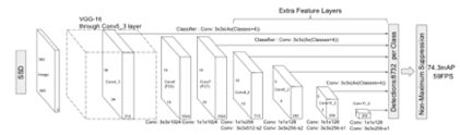
This is the architecture of the Single This is the Single Shot Multibox Detector. It has multi-scale feature maps which decrease in size progressively and allow predictions of detections at multiple scales. Each added feature layer can produce a fixed set of detection predictions using a set of convolutional filters.

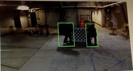
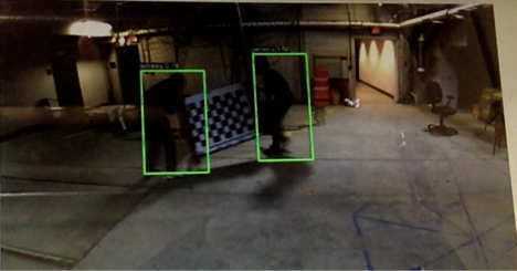
The following pictures are the results for the real-time detection.

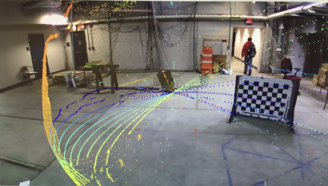
Camera-Lidar Calibration:

I recored several bag files using the camera and velodyne with /zed/rgb/raw_image topic and /raw_points topic.

Setup the Autoware Calibration toolkit which looks like this.

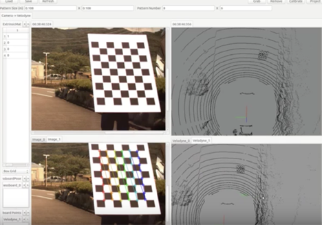
Grab some frames from the toolkits and manually label the corresponding location of the point cloud given the images. However, the result is not impressive (See the following picture).

The reason why the distortion is so bad is because I didn’t grad enough frames. It requires 60 camera-velodyne frames in different angles, locations to reach better performance. Our calibration board is too heavy to move so that I decide to use other calibration tool kit to proceed the task.