Vehicle
Our vehicle subsystem for the is a miniature autonomous vehicle built by the D team last year3. We have also outfitted the vehicle with a thin wire “bumper” to increase the scale in relation to humans. The vehicle is built with a chassis from a hobby RC car and is controlled with an onboard Jetson TX1. The TX1 connects to a Teensy microcontroller which commands the vector electronic speed controller (VESC) that controls the motors of the vehicle. It also connects to a passive wireless receiver, Hokuyo LiDAR, USB hub, IMU, and power distribution board (PDB). The PDB receives power from an 11.1V lithium polymer battery and distributes it between the active components. The vehicle can be seen in figure 1 below.
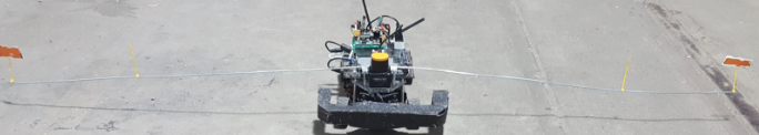
Figure 1 – Vehicle subsystem
The ROS visualization tools provide an excellent view of how the car’s subsystems work together to produce a working system. The rqt_graph of the fully functional system can be seen in figure 2 below.
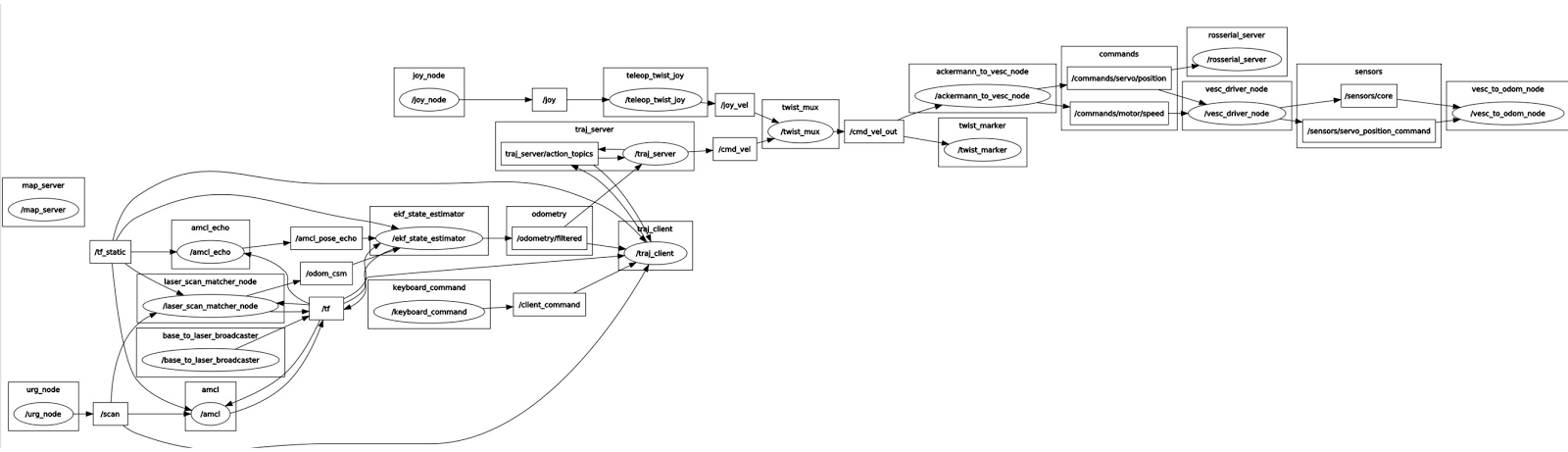
Figure 2 – vehicle rqt graph
The bottom left of this rqt_graph shows how the IMU and laser scanner feed into an adaptive monte carlo localizer (amcl), then into a an extended Kalman filter to provide state estimation4. This information is published as odometry information which is used by both the trajectory server and trajectory client. The trajectory server sends commands through the multiplexer to the Ackermann controller, which controls the motor and steering. Left out of that description is the keyboard command, which feeds into the trajectory client. The command a activates the ramp protocol, which moves the vehicle to user-defined goal point. Specifically, this references a yaml file (bsilqr_params.yaml) which has a predefined goal location (along with other parameters). This planning method is executed by the trajectory client and server, which utilize the ROS action library to steer the robot to the goal.
Missing from the above graph is the connection to our infrastructure. When working together, the trajectory client subscribes to the “/predicted_points” topic which carries the PoseArray message that contains pedestrian trajectory data. The trajectory client includes a node that will stop if this pedestrian data is determined to be in the vehicle’s path.
By connecting to a ROS core running on the vehicle’s TX1, we are able to view the “odometry_filtered” and “scan” (from the Hokuyo) topics on the vehicle’s map. Since the system came pre-built, we did not perform any modelling on the vehicle.
The analysis came in a rigorous poring over of the ROS nodes when the vehicle was active to determine how the subsystems worked together. Since our communication needed only to interface with the trajectory client, contained within the “ilqr_loco” package, this package was the primary area of focus. Toward the end of the semester, when we started interfacing with the infrastructure more regularly, the ekf used for state estimation was analyzed as well.
We performed extensive testing on the vehicle in order to perform our fall validation experiment without failure. What you can see in figure 3 below is the vehicle’s odometry with respect its initial position (odom frame), the velodyne frame, and a human in its path.

Figure 3 – Vehicle running in rviz
The ability to visualize the vehicle was useful for the many iterations we performed changing the map of our test environment, running the vehicle to its waypoint, and testing the vehicle with live pedestrians. Primarily, this feature made it easy for us to determine where the vehicle believed it was with respect to the environment and the LiDAR.