Spring Semester Updates

The two major components of the project for the spring semester are the Navigation sub system and the Estimation sub system. This section covers the progress made in both the sub systems.

1. Navigation

1.1 Advanced Base Construction

We choose to go with in-wheel hover board motors for the motorized upgrade of the SoyBot. The detailed trade study can be found here. Additionally we designed a new mount/adapter for these motors. Next the entire assembly was integrated with the SoyBot chassis.

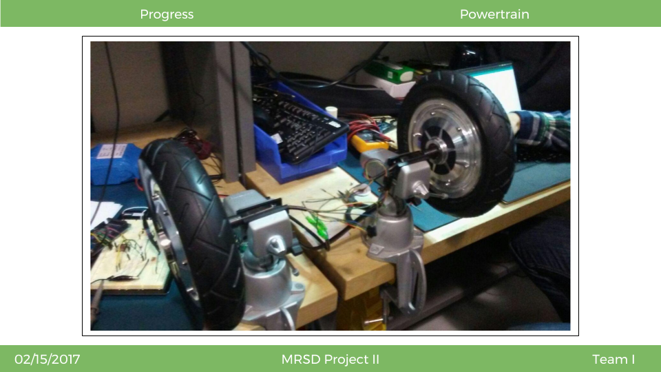
Figure 1.1 In-wheel motors

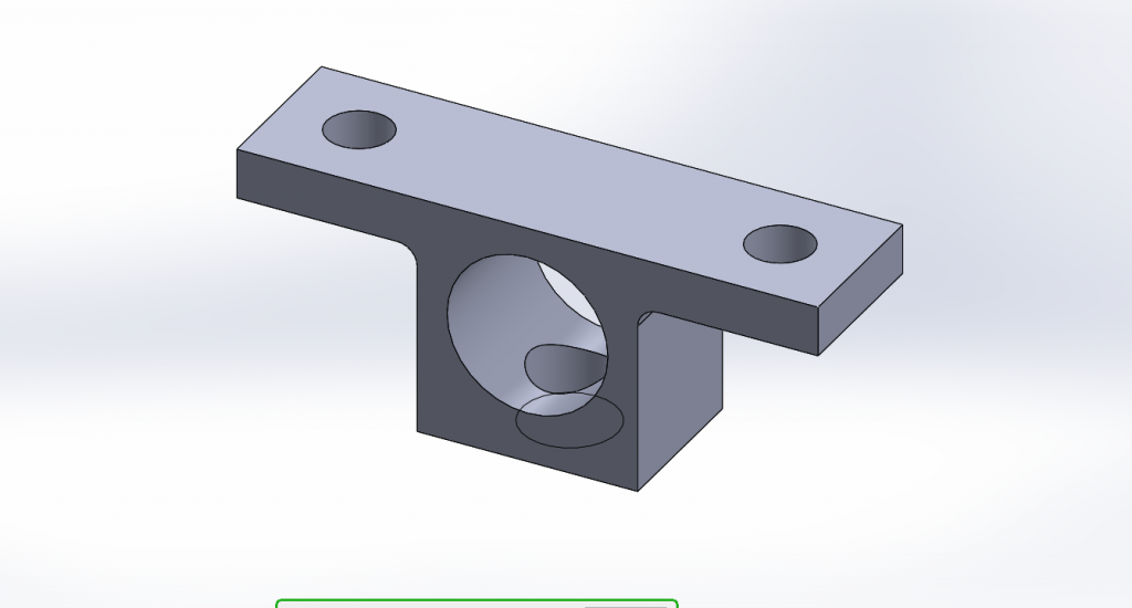
Figure 1.2 Motor Mount/Adapter for in-wheel motors

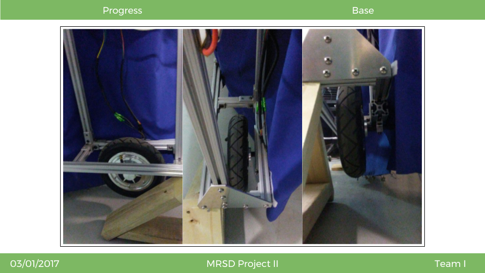
Figure 1.3 The new motorized wheels have been mounted onto SoyBot with the new adapter

1.2 Power Train

The new drive power train is also mounted on SoyBot. Each wheel is powered by one 36V 4.4 Ah battery. Each wheel also has its own motor controller board and arduino interpreter to decode messages and interface with the main vehicle computer.

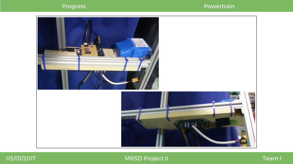
Figure 1.4 Power Train for SoyBot

1.3 Sensors and Calibration

The two sensors that will be used for navigation have also been fully integrated with the vehicle. We are using two lidars facing at a 45 degree angle down at the row of plants to assist with high level navigation planning. The three scenarios that we will be dealing with are shown on the right. The vehicle can be partially in the row where only the front lidar is used, fully in the row where both lidars are used, and leaving the row where only the back lidar is used.

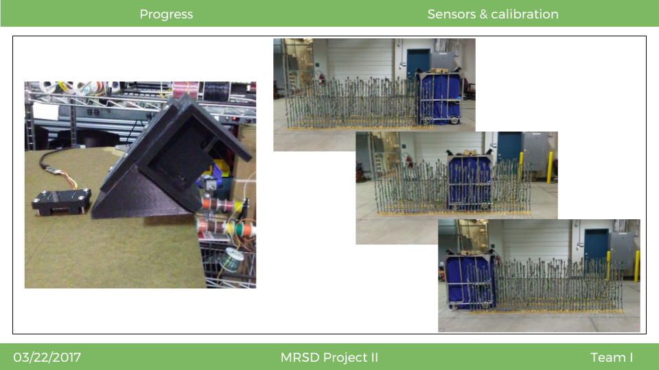
Figure 1.5 Navigation Sensors for SoyBot

1.4 Localization

This video shows a test run of autonomous navigation with one lidar through a 6+ meter long row of plants. We are using RANSAC and additionally filtering based on the geometry of the lidar position to fit 3 lines to the rows, shown in blue. We then use these three lines to get an estimate about where the vehicle is with respect to the center row, shown as the yellow arrow.

1.5 Controls

The main idea for this control system is to map the vehicle offset from the center row of beans, to a target orientation for the vehicle. Intuitively, this means that target orientations will be smaller angles when the vehicle is close to the center row, and larger angles when the vehicle is far away from the row. Right now the lidar is providing feedback and giving an estimated pose of the system including orientation and position with respect to the center row of plants. From the feedback of how far away the vehicle is from the center of the row, a target orientation of the vehicle is generated. At that point a traditional feedback control system is used with a proportional controller. The target (reference) orientation is compared with the actual orientation of the vehicle, and then fed to a controller to send an angular velocity command to SoyBot.

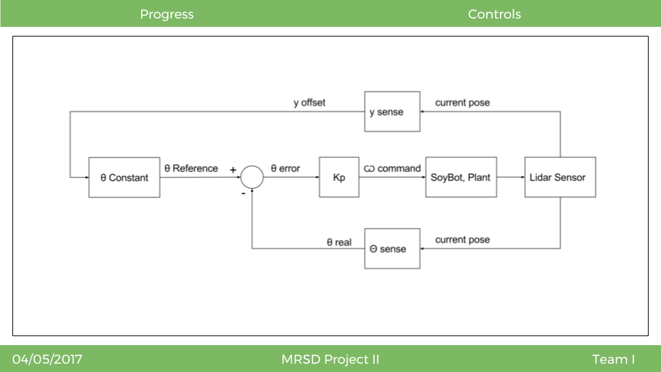
Figure 1.6 SoyBot Control System Outline

2. Estimation

Figure 2.1 illustrates the high-level navigation architecture. The sensors array consisting of four point grey chameleon cameras (see section 1.1 in Fall semester system status) capture raw plant data. This raw data is processed and undistorted using the camera calibration model. Next the pod detection and pod tracking modules are deployed to get a pod count per camera. After we get the count per camera, we use the sensor model calibration parameters to fuse the pod counts from each individual sides (vertical integration ) followed by fusion of counts from all four cameras (Global integration).

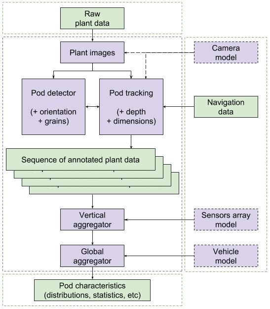
Figure 2.1 Estimation Architecture

The pod detection and identification

• Detection & Description/Segmentation : Detect each individual soybean pod in anindividual frame
• Registration & Tracking : track every individual pod across frames
• Registration & Side Matching : match the pods detected from images captured by both sides of the sensors array.
•  Depth, 3D & Dimensions : Get depth (2.5 D), pod dimensions and 3D reconstruction of the soybean plot.

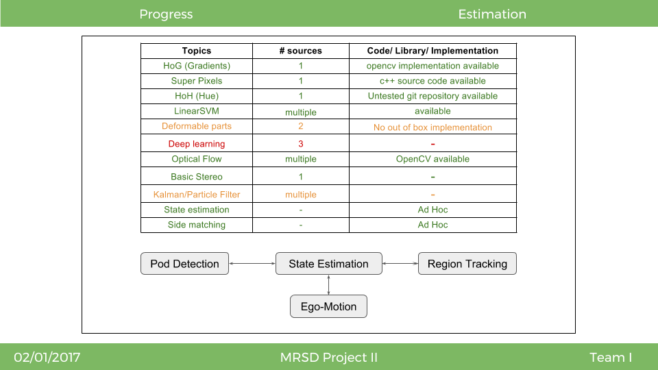
Figure 2.2 Estimation pipeline

2.1 Pod Detection

The detection module uses Histogram of Oriented Gradients (HoG) and Histogram of Hue (HoH) as the features for identifying the soybean pods. These features are normalized and fed to a Stochastic Gradient Descent Classifier to get a prediction. The prediction is clipped at a threshold (which is a hyper parameter), to get our candidate soybean pods. Next we run a local maxima search to find peaks, which depict the final detection.

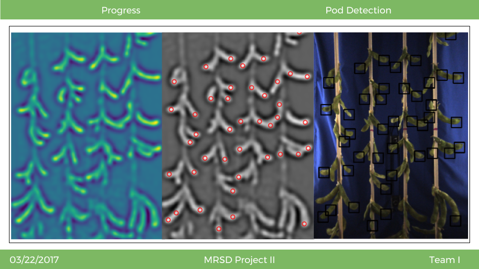
Figure 2.3 Pod Detection Module Results, (Left to Right) Detection Heatmap, Detected Peaks, Bounding Boxes for detected soybean pods

The pod detection module has five hyper parameters, viz. cell size, block size, detection threshold, min distance between detections and a Difference of Gaussian filter sigma values.  We did an initial parameter sweep for the cell and block sizes. Figure 2.4  shows the qualitative results across these parameters for cell and block size set to 6,7,8, and 10. All the other parameters were fixed (threshold = 0.35, min distance = 5px, sigma min = 1.5 and sigma max = 2.5)The preliminary parameter sweep was essential to detect failure cases. One of the prominent failure cases observed had the soybean tip having the stalk and/or ground in the background.

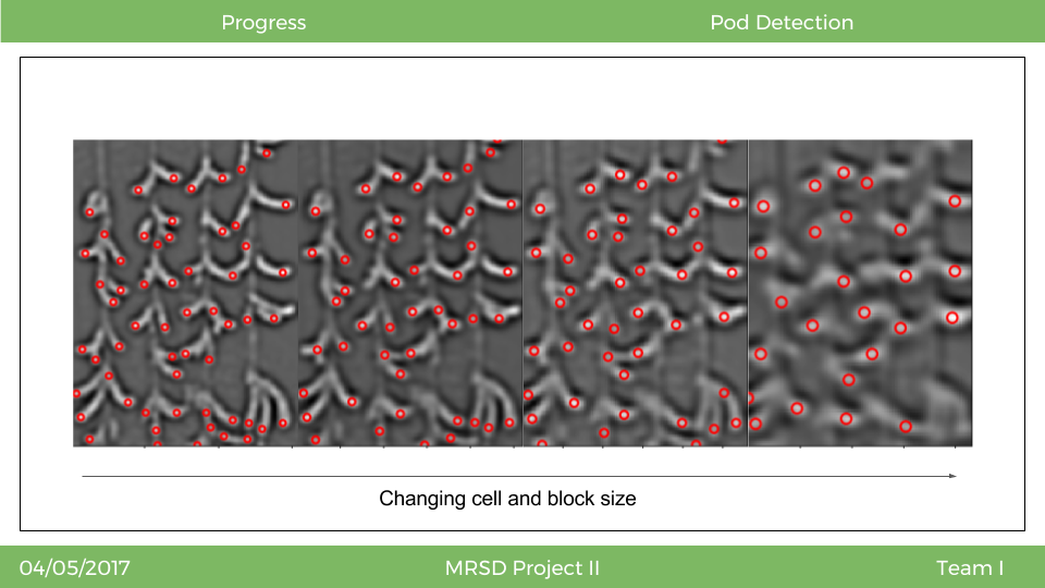
Figure 2.4 Parameter sweep with cell and block size set to 6,7,8, and 10 (Left to Right)

We also implemented a method of filtering our detections. The central idea for this approach is to eliminate duplicate detections for the same soybean pod. Figure 2.5 illustrates the result for this process. The left image highlights some of the duplicate detections while the right image shows the results after we filter the duplicate detections. The green contours demonstrate the successful cases while the blue contour demonstrates the case where this method fails. To counter the failure cases, we added a minimum lateral distance parameter which would prevent discarding overlapping pod detections (which is one of the failure cases).

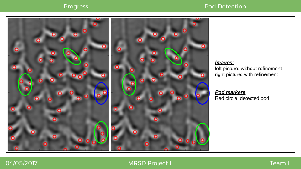
Figure 2.5 Results for Refine Peaks;  Green contours: successful cases; Blue contours: Failure cases

2.2 Pod Tracking Module

The pod tracking module tracks individual pod detections across multiple frame to enable counting the soybean pods correctly. Figure 2.6 shows the results for tracking a single bounding box across multiple frames. Figure 2.7 shows the results for fusion of tracking results from the top and bottom cameras on a single side of the sensors array. The initial pod count results are illustrated in figure 2.8 (No vertical or global integration was accounted for getting this pod count).

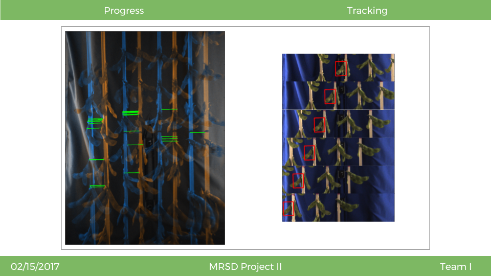
Figure 2.6 Tracking a single soybean pod across multiple frames

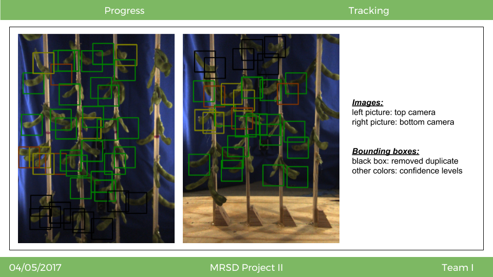
Figure 2.7 Pod Tracking module results, tracking multiple pods across multiple frames from 2 cameras on the same side.

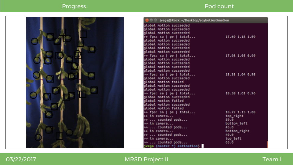
Figure 2.8 Initial Pod Count results (without vertical and global fusion)

Fall Semester System Status

Figure 1.1 outlines the work break down structure for the project based on the sub systems. As illustrated by the figure we have 5 main sub systems for the project viz. the sensor array, Mechanical Platform, Onboard Electronics, Integration and Estimation Subsystem.

Figure 1.1 Current Implementation status (Fall System); Green : Completed, Yellow: In progress; Red: Not Started

1.Sensors Array

1.1 Cameras

The choice of camera was based on a trade off between the following factors:

• Sensor
• Sensor size
• Resolution
• Pixel size
• Dynamic Range
• SNR
• Frame rate

The Lens was chosen based on the following factors:

• Depth of focus
• Field of view

Distortion, pixel density, footprint, trigger, total throughput were the other considerations for the choice of the cameras. Based on all these factors we chose the Point Grey Chameleon 3 cameras and the Aercont 2.8mm 1.3 MP lens. The USB 3.0 hub was chosen to support the required bandwidth of the data we need. The complete analysis can be found here.

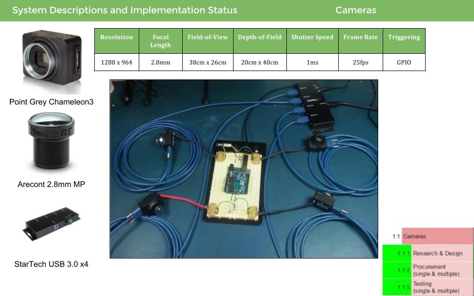
Figure 1.2 Point Grey Cameras, lenses, USB Hub

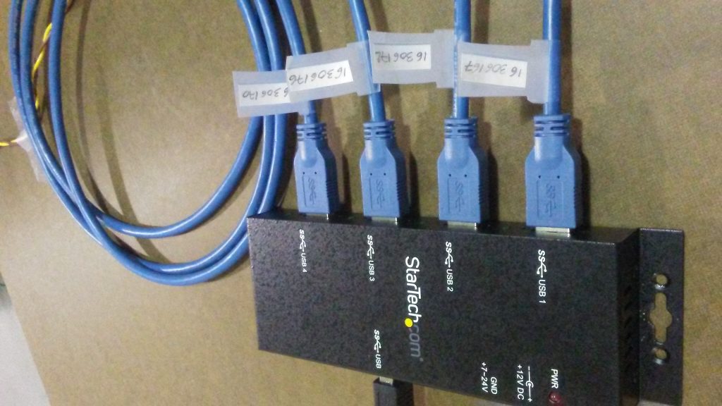
Figure 1.4 USB 3.0 Hub

1.2 Lighting Sub System

Based on the power constraints of our system, we chose to go ahead with led strip lightning. Three parameters were decided to make this choice viz. Lumens/ft. , Lumens/Watt and Lumens/dollar. We selected the last option because it has a very high advantage in the Lumen/W and Lumen/$ parameters although it isn’t as bright as one of the options on the list.

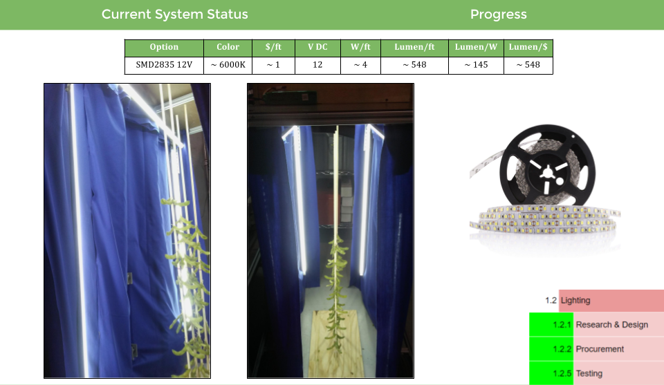
Figure 1.5  Lightning Sub System

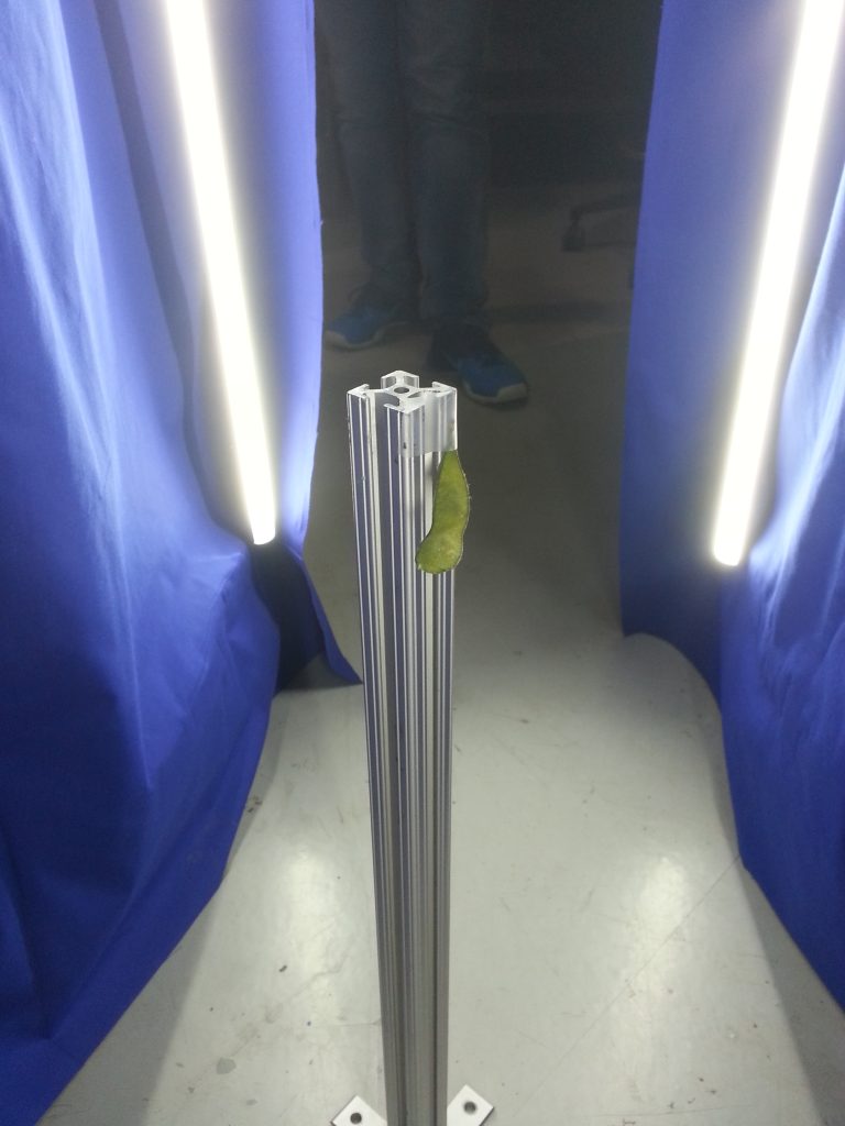
Figure 1.6 Lightning Test setup with the SoyBot

    1.3 Test environment

The test environment setup for the fall semester is going to be a combination of calibration targets and soybean pods mounted on wooden stalks.

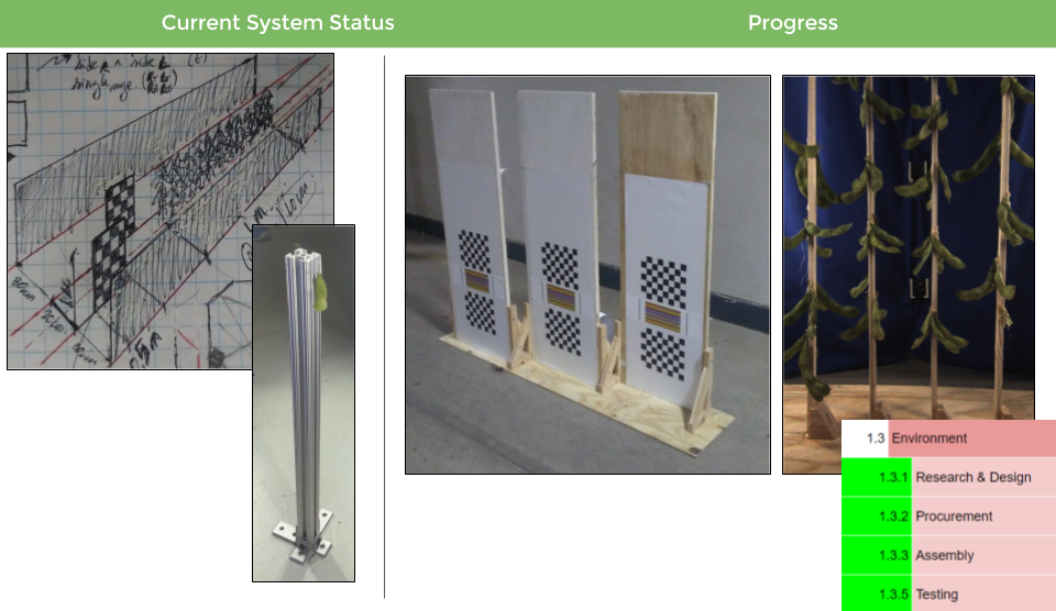
Figure 1.7 Test Environment

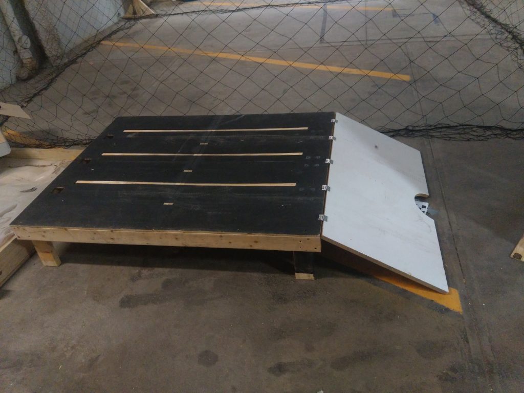
Figure 1.8 Ramp setup for SoyBot Demonstration

1.4  Advanced Test environment

The advanced environment will consist of 3 rows with a single row of stalks with soybeans and 2 rows on each side of the center row with just the stalks. the total length of the test field will be 3 meters.

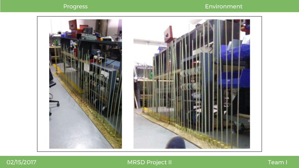
Advanced environment

2. Mechanical Platform

1.1 Chassis

The chassis of SoyBot is built out of 80/20 extruded aluminum for ease of assembly and reconfiguration. The general shape is an “inverted U,” which allows plants to move through the robot and take pictures of both sides. It will fit between standard-sized rows of soybeans and will accommodate plants up to 1.2 meters high. Electronics and the user interface will be mounted on top.

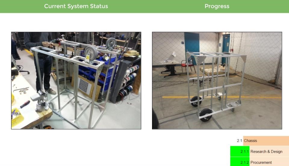
Figure 1.9 SoyBot chassis

2.2 Sensor Support

The sensor array is supported by a vertical piece of 80/20, which is attached to the rest of the chassis with rubber vibration dampers. The cameras are attached to the sensor support with custom mounts made on the 3D printer.

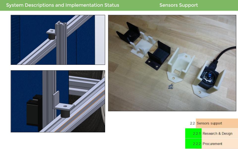
Figure 1.10 Sensor Support system

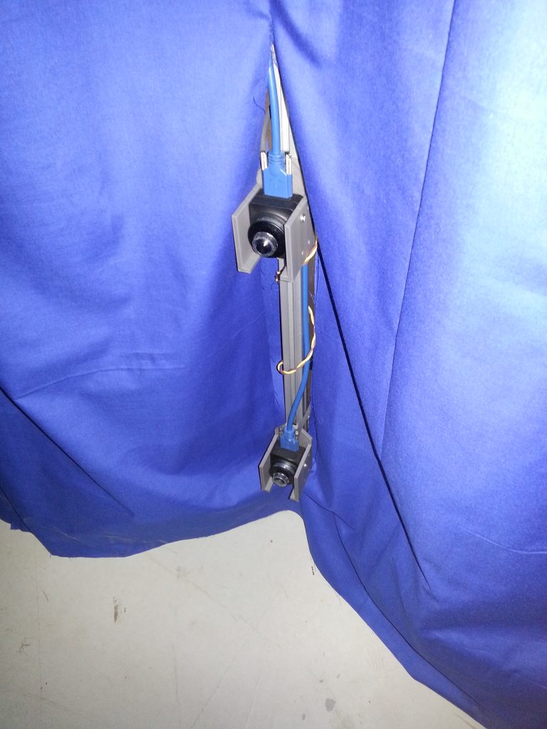
Figure 1.11 Camera mounting

2.3 Simple Base

For the fall semester, we are building a simple version of the base, which consists of two large pneumatic wheels in the rear and two rubber casters in the front. This will allow the vehicle to be pushed through the testing environment for the fall validation demo. A powered base with motors and steering capabilities will be used for the spring semester.

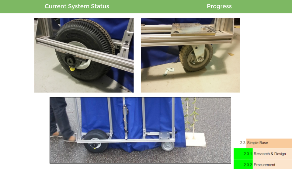
Figure 1.12 Simple base for SoyBot

2.4 Initial Platform

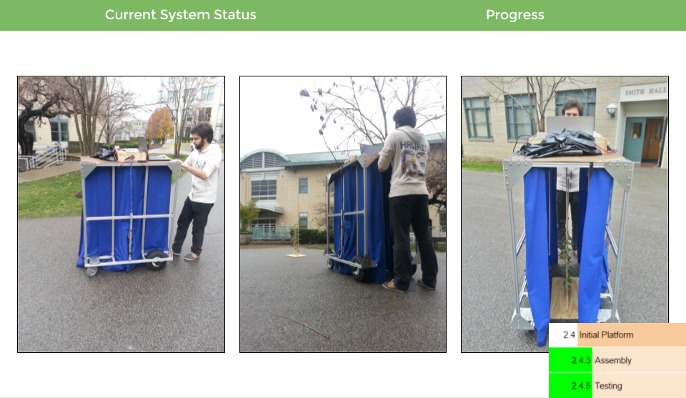
Figure 1.13 Completely fabricated initial platform

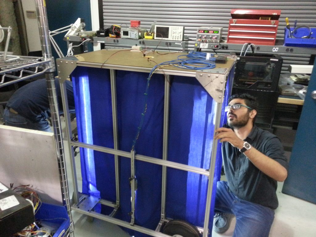
Figure 1.14 SoyBot work in progress

3. On-board Electronics

3.1  Acquisition and Storage

•  The system will have a data rate of at least 176 MB/s which is equivalent to four Chameleon 3 Point Grey Cameras running at 25 FPS
•  The system shall have adequate GPIO to trigger the cameras and interface with other systems if needed
•  The system will have at least 64GB of storage space for at least 5 minutes of data acquisition

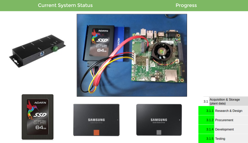
Figure 1.15  Acquisition and storage system with Nvidea Jetson SBC, USB 3.0 HUB and SATA SDD

3.2 Power Distribution

Assumptions/Constraints:

• Limited by Eagle CAD software for assignment

• Limited by Eagle CAD board space for assignment

• Limited by manufacturability  TH mount was mostly chosen or decent size SMD.

• Limited by time, extensive research was done to find the correct regulators but the passive components were not well researched and more optimal choices might be available.

• Limited by lack of knowledge of motor voltages and powers, expensive and wide range regulators were chosen for this reason.

• Limited by lack of knowledge of the end number of interfacing components. Lots of extra connectors were added and the regulators have larger current output than the minimum just in case we need more systems for navigation/motor interfacing in the spring

• Limited by lack of knowledge of battery voltage. The PDB is designed so that there is flexibility with the input

Design Reasoning

From the above assumptions and constraints, the general design choices were for modularity and ease of manufacturing.

Future considerations

For future iterations with well-defined subsystems I suggest narrowing down the exact connections needed for the system and replacing the voltage regulators with cheaper, more optimal components that satisfy the predicted voltage/current range of the system.

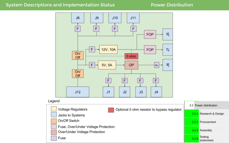
Figure 1.16 Power Distribution Board Schematic

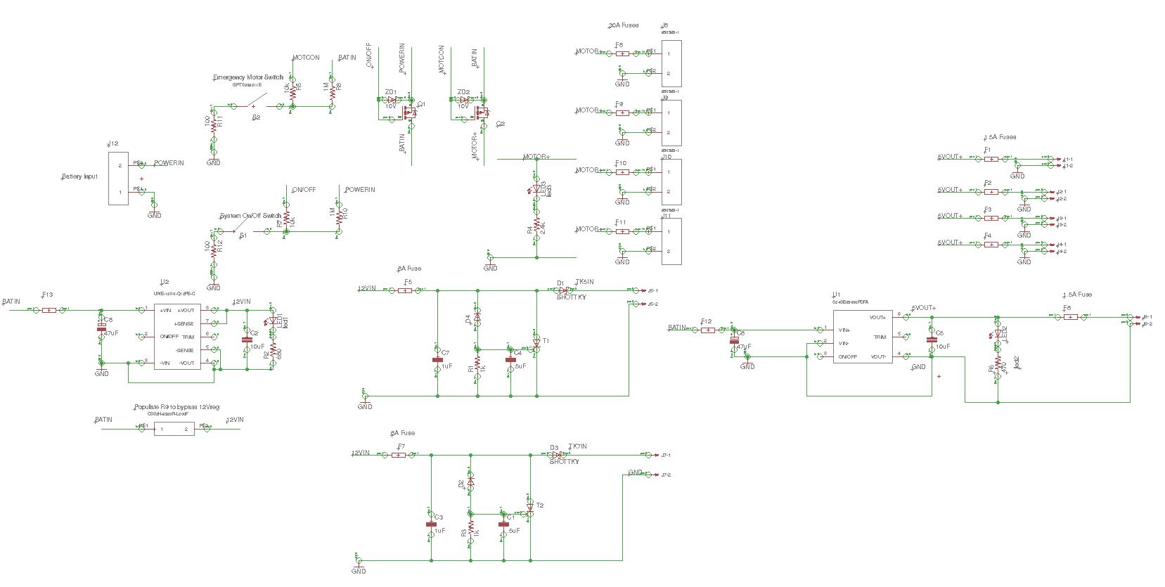
Figure 1.17 Power Board Schematic

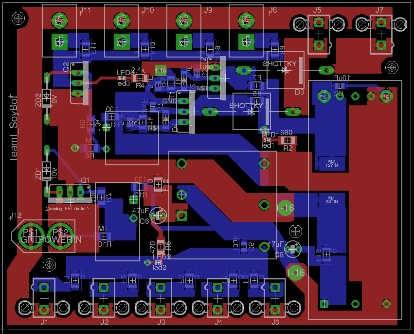
Figure 1.18 Power Distribution Board

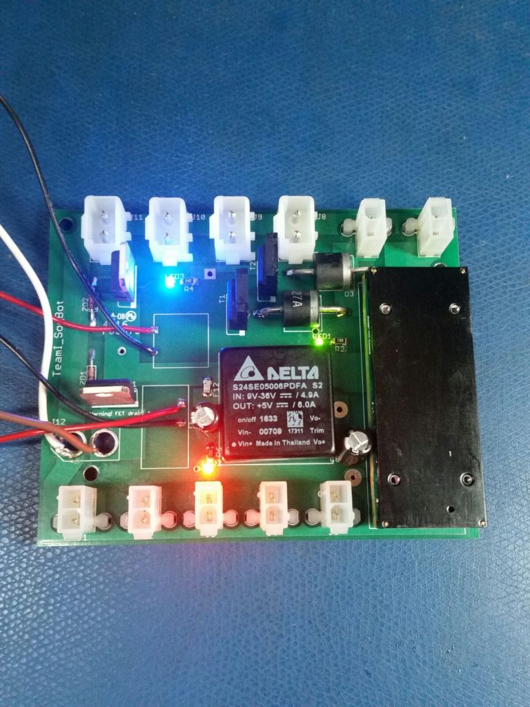
Figure 1.19 Final Assembled Power Distribution Board

3.3 Onboard (ROS) Interface

The first and lowest layer of the sensors array is defined by the PGRCamera class, an object-oriented abstraction of the flycapture SDK provided by Point Grey. It allows for easy, encapsulated programmatic control over settings, configurations, and overall behavior of any Point Grey camera (compatible with the SDK) over a USB 3.0 bus. We will not (extensively) use the images online, i.e. while the robot is moving, since we only want to store them for later use and we do not want to clutter the network bandwidth with over 200MBps of unnecessary data. The second layer of the sensors array is defined by the Grabber class, built on top of the PGRCamera class. There are multiple instances of the Grabber class during run-time, one for each camera. The purpose of a grabber is to provide a control interface for the camera to the rest of the ROS environment. After configuring itself and the camera associated with it using the parameter server, a grabber will wait for an image to be transmitted from the camera and then potentially pre-process it, save it to disk, and/or stream it over a topic at a lower rate. The third and last layer of the sensors array is comprised by the Photographer class which is instantiated as a singleton. The photographer is responsible for triggering the cameras, either by software or by hardware.

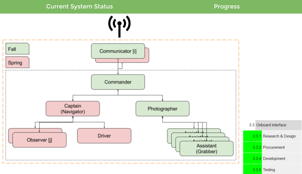
Figure 1.20 ROS interface layout

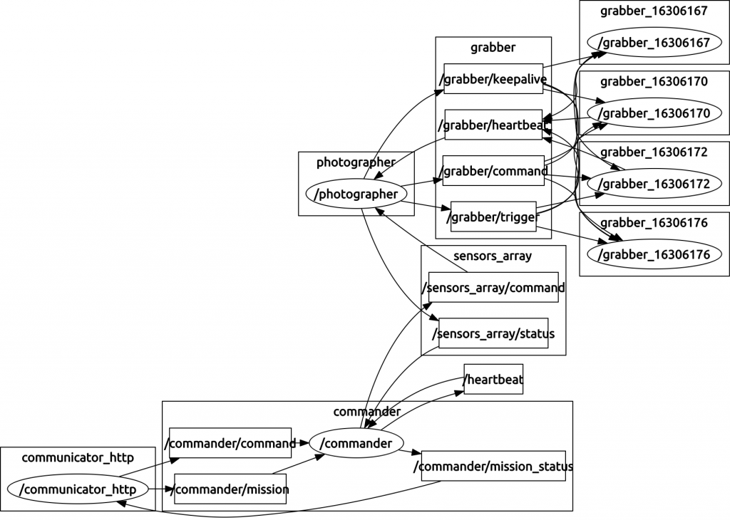
Figure 1.21 ROS Graph

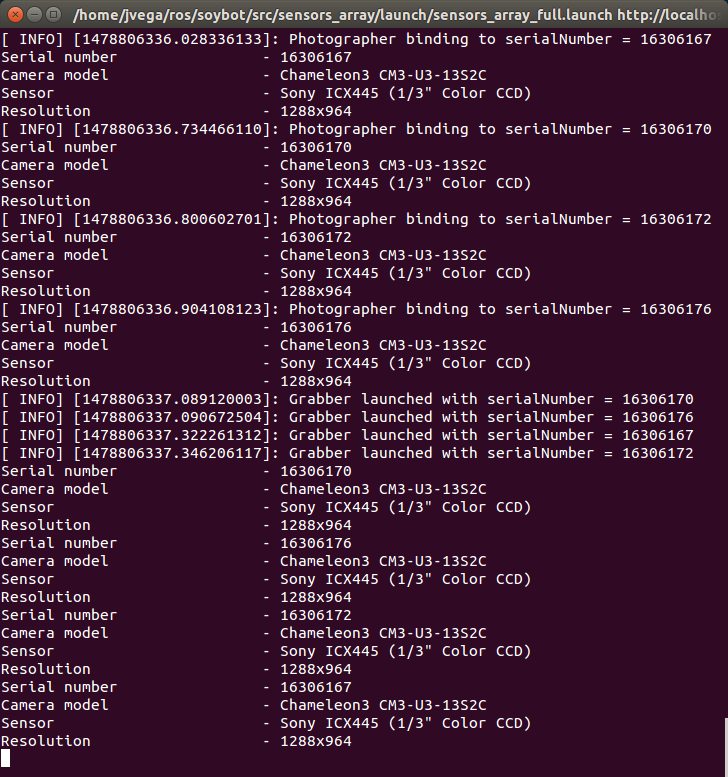
Figure 1.22 ROS interface for multi camera setup

4. Integration

4.1 Input Visualization

Once we have collected all the images, we need a convenient way of showcasing the 3 main performance parameters we set to achieve for the FVE viz. Horizontal Overlap, Vertical Overlap and Pixel Density. Figure 1.3 presents a high level layout plan for showcasing all of these parameters.

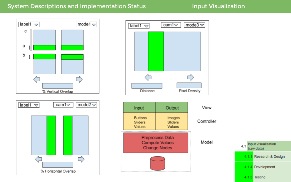
Figure 1.23 Input visualization schematic

The Visualization subsystem resides on a remote computer. We are using PYQT library  in python to create the GUI. We have 3 windows one each for the 3 parameters we want to measure. Figure 1.5 shows the window for calculating vertical overlap between two images. We have 4 cameras in our system, 2 on each side. The 2 cameras on each side have an effective vertical overlap and we want to be able to calculate the overlap. We draw 2 horizontal lines which can be dragged on the image using the slider. The idea is to match a line on both the images (vertically). As illustrated in Figure 1.3, we have 3 variables a, b & c. The effective vertical overlap is given by the quantity (a + b)/c.

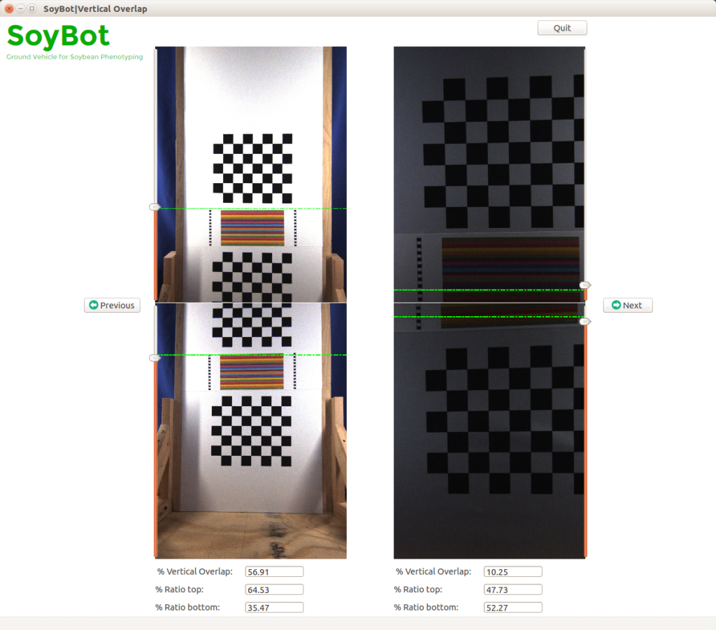
Figure 1.24 GUI for Vertical Overlap

Horizontal overlap is the overlap between 2 successive images captured by the same camera. Assuming that the scene doesn’t change between 2 consecutive shots, horizontal overlap can be calculated using the same ratio (a + b)/c. (see Figure 1.4).  In this window we have a choice of camera which is a simple dropdown list.

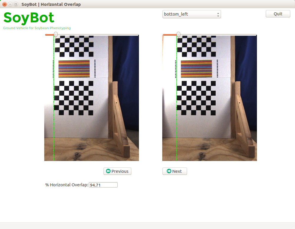
Figure 1.25 GUI for Horizontal Overlap

Pixel density is the number of pixels packed per unit area of an individual image. The user slides two parallel vertical lines on the image and inputs the actual measured  distance between the 2 lines. The GUI gives the actual density of the pixels between these 2 lines. The user can choose from the list of cameras and go back and forth between images.

Figure 1.26 GUI for displaying Pixel Density

5. Estimation

5.1 Calibration

Camera calibration is used to find the intrinsic characteristics of the camera viz. camera matrix and distortion coefficients for the camera and lens setup. We used OpenCV for coming up with these parameters. A chess board pattern was used to do the calibration. We used multiple setups for calibration. First up a test rig was used to get the camera calibration parameters. Later we used our SoyBot setup to calibrate the 4 cameras.

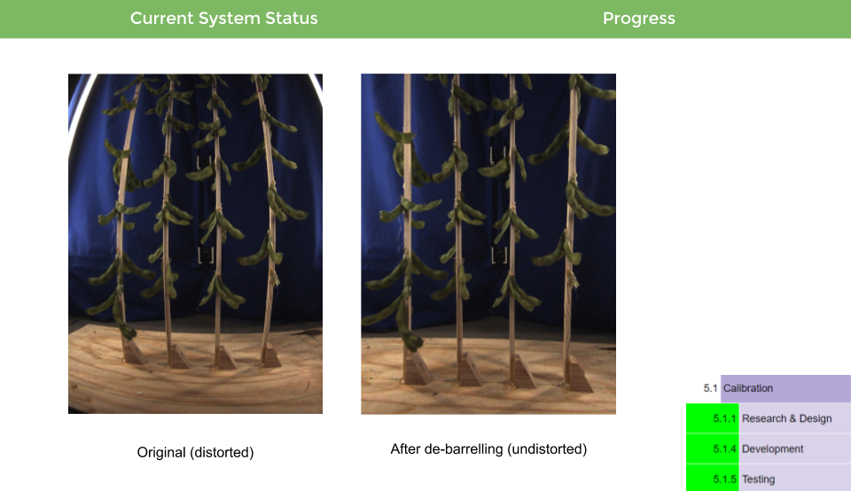
Figure 1.27  Camera calibration results