Implementation

Fall ’16

---

Our system was initially envisioned to be a pair of mobile robots which would track the user’s gait and position themselves to capture the feet as they land, hence providing a firm ground feel while moving the user back to the centre. Figure 1 shows a representation of the concept.

 

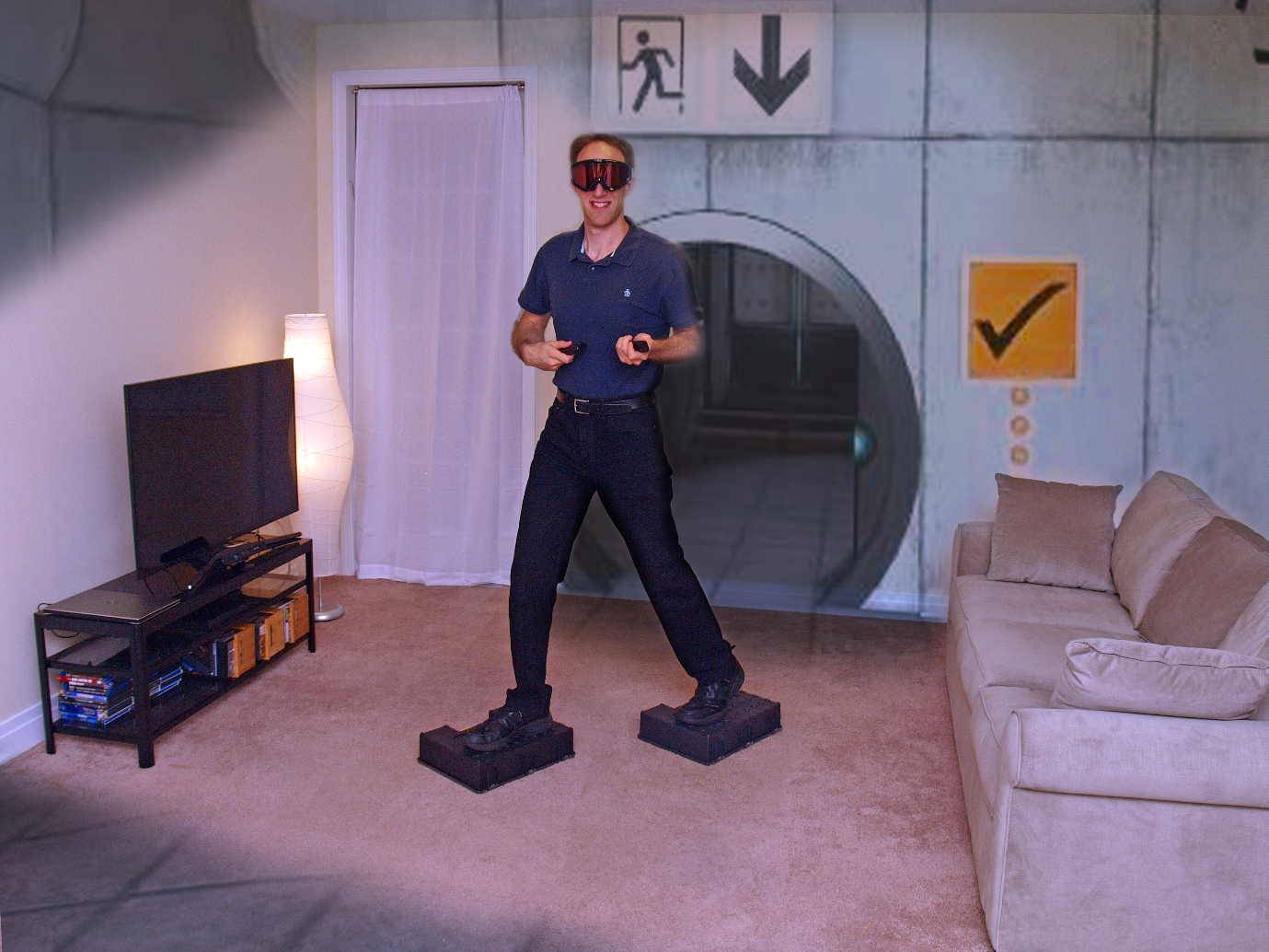
Figure 1: Initial concept

We studied human motion capture data and drew up some plots of the displacement (relative to the sacrum), velocity, acceleration, and forces associated with human gait. These plots are seen in Figure 2 for both feet.

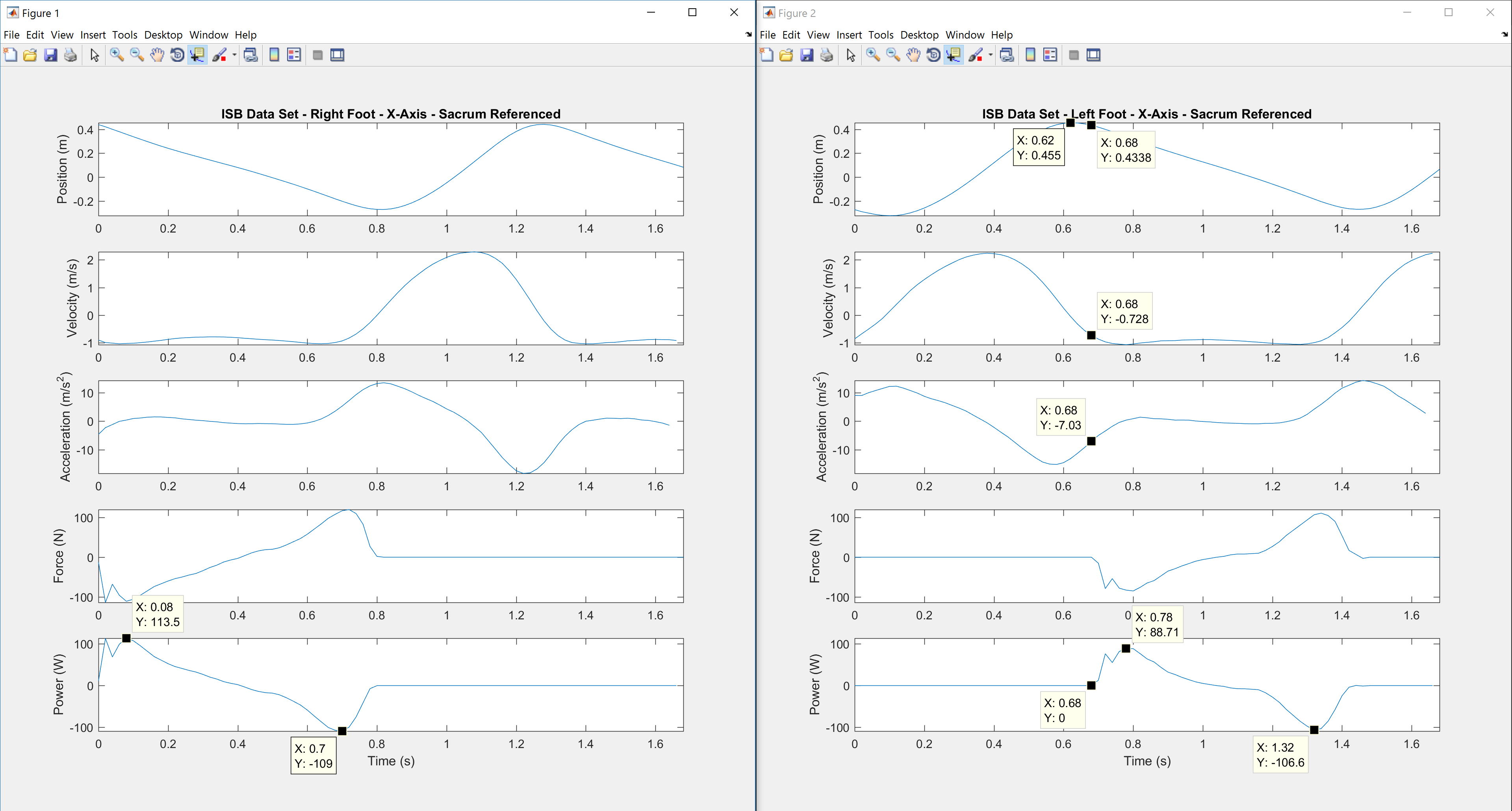
Figure 2: Foot characteristic curves during gait

From analysing the data, we concluded that the above mobile platforms concept is infeasible due to acceleration requirements. For the mobile platforms to position themselves to capture the user’s feet, they must be at least as fast as the average foot velocity, and this would require accelerations larger than g (9.81 m/s^2). Any robot driving itself through friction with the ground is limited in its acceleration to a value of u x g, where u is the coefficient of static friction. In practical cases, this coefficient is smaller than 1, which implies that a robot cannot exceed an acceleration of g. Hence we had to pivot to a different concept.

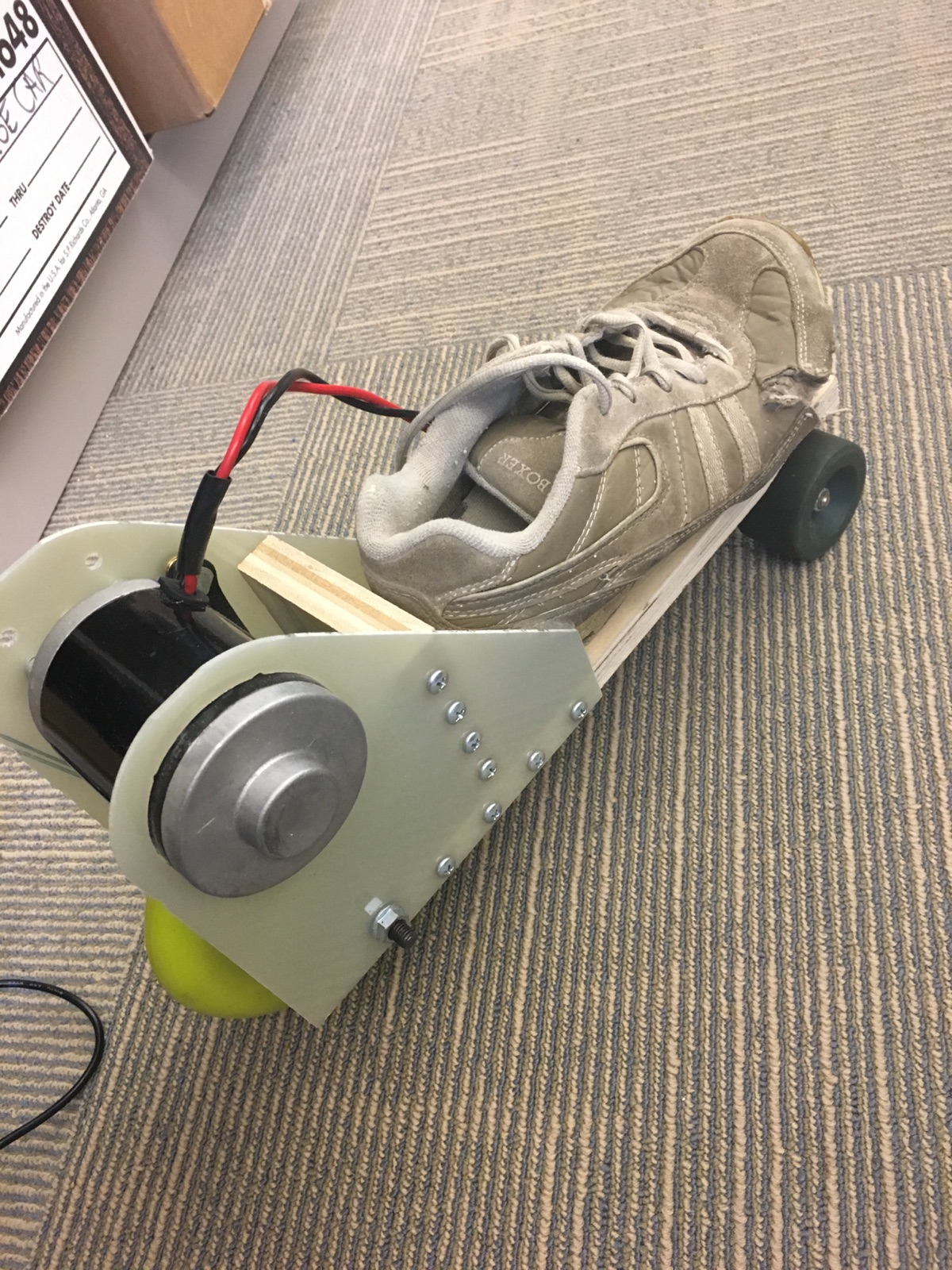
Figure 3: Nimbus shoe prototype

Taking inspiration from an electric powered skates project (Figure 3) at CMU pursued by Ph.D. student Xunjie Zhang under the guidance of our mentor Dr. Chris Atkeson, Team Morpheus decided to pivot to a similar idea, the main difference being that the primary function of the skates is to re-centre the user rather than push them along.

The system comprises of 3 major subsystems –

1. Powered Skates
2. Unifying Sensing and Control
3. Visual-Audio VR

 

Subsystem 1: Powered Skates

The first iteration of the mechanical structure of the skates was completed ahead of FVE. The design consists of over 35 unique parts either designed from scratch or selected to serve a specific purpose, and well over 100 combined instances of these parts per skate.

The manufacturing of these various parts was split between various machining techniques and 3D printing. Having gained access to the National Robotics Engineering Centre’s waterjet cutters and CNC lathes (thanks to Dr. Dimitrios Apostolopolous), parts of the system like the drive shaft, the motor-gearbox adapter, and the top plates were machined with relative ease. The rest were manually machined in the Robotics Institute’s machine shop at Carnegie Mellon University. The material used was 6000-series Aluminium alloy stock. Some of these parts are seen in Figure 4 (below).

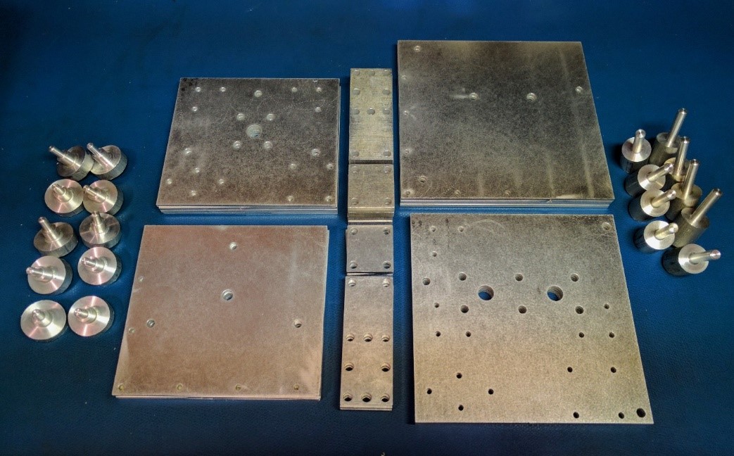
Figure 4: Parts machined at NREC using CNC lathes and waterjet cutting

A sizeable number of parts, like the mounts for the gearbox, the bearing, and the ball caster units were 3D printed in PLA. Using a higher in-fill of 50-70% achieved the required strength in this application. A batch of 3D printed parts is shown in Figure 5 (below).

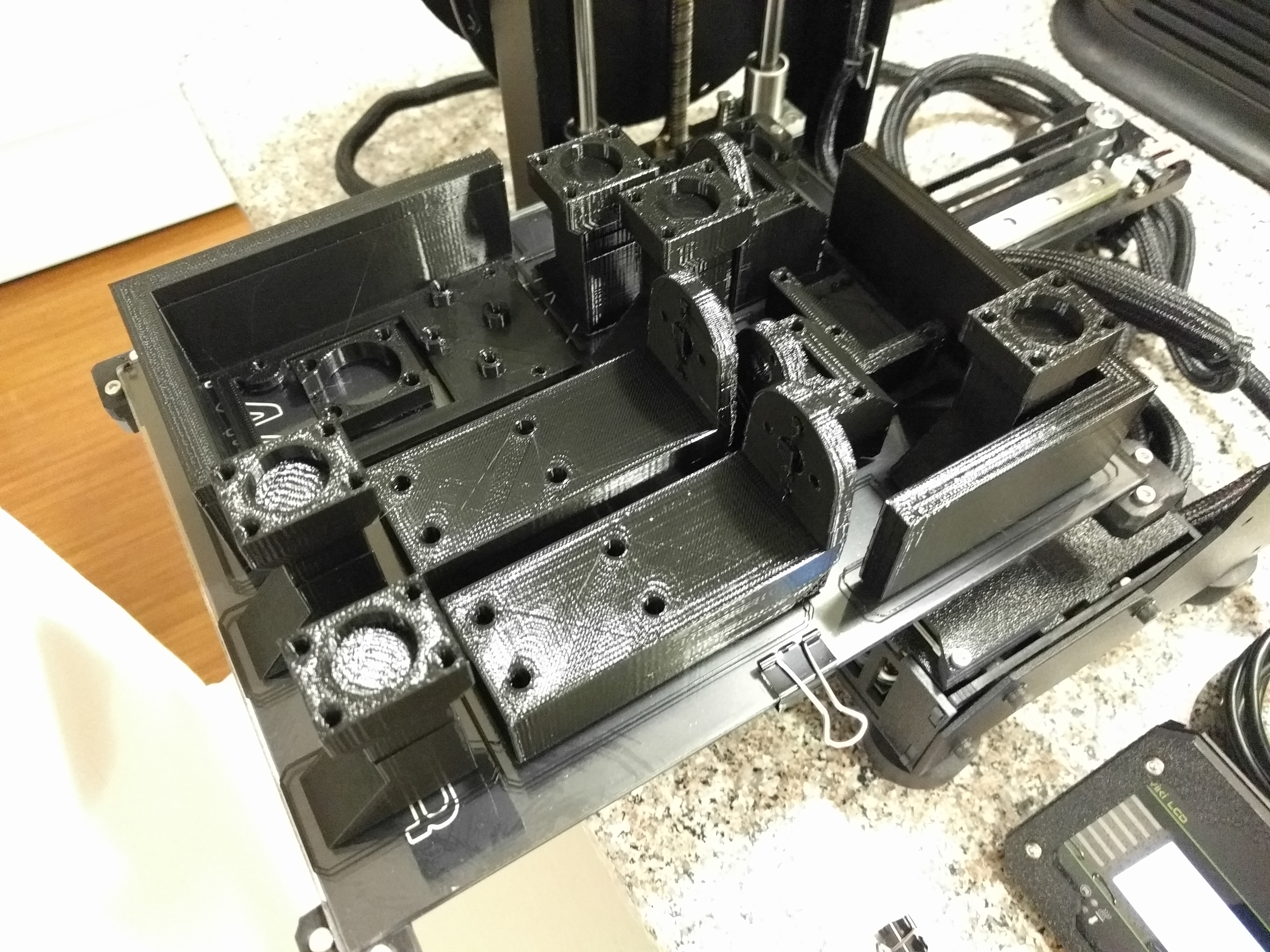
Figure 5: A batch of 3D printed parts

The rest of the hardware was acquired from a variety of online vendors, most notably McMaster Carr. The design of the skates accommodated a degree of freedom in the middle (hence each skate was split into 2 halves) to allow for more natural gait and preserve the flexibility of the human foot. The skates, fully assembled, can safely handle weights up to 90 kg.

                   

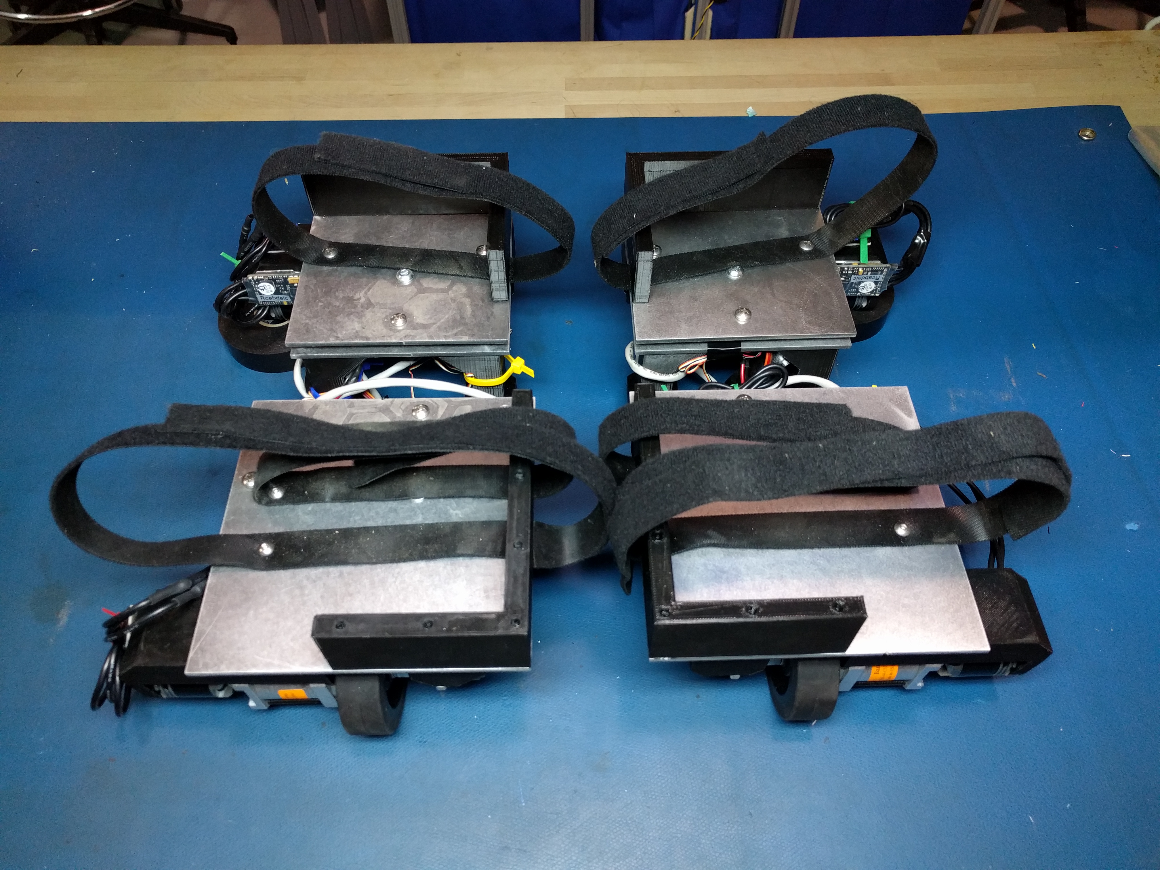
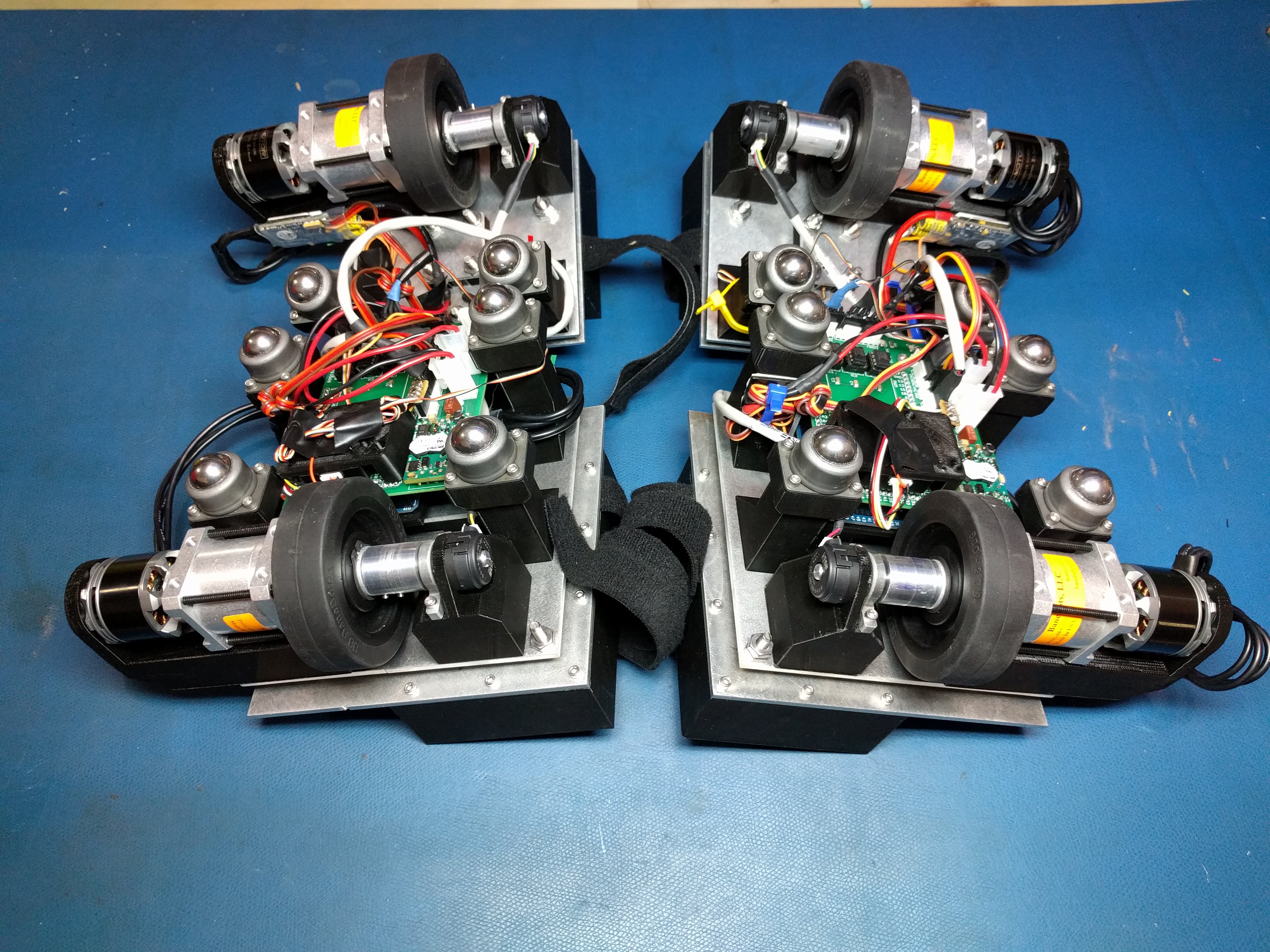
Figure 6: The fully assembled skates

The power distribution board was used to supply power to the on-board sensors and to provide a relatively robust connection to the Arduino. The board was designed to act as a stackable shield with the Arduino, and worked reliably during the Fall Validation Experiment and the Encore.

The main shortcomings of the sub-system were –

• The absence of a suspension for the front-half of each skate, and the sub-optimal placement of the drive wheels resulted in insufficient traction on these wheels for some user weight ranges.

• The front and rear halves of the skates tended to misalign over prolonged use.

• The electrical connections to the PDS PCB were not sufficiently robust.

 

Subsystem 2: Unifying Sensing and Control

I. SENSING

There are four main sensing components, each of which corresponds to a particular system requirement. The optical encoders, which are used as a part of the control loop for velocity and position control and tie in to requirements MPR1 and MPR2. The Kinect provides a point cloud and skeletal key-points which ties into both the aforementioned system requirements. Each powered skate has an inertial measurement unit on it to indicate position and velocity which would further consolidate the first walking requirement and is also a step towards being capable of supporting walking in different directions. Force sensitive resistors are placed at the ball and heel of each foot to indicate the position of the centre of pressure for balance and whether the subject is walking or standing; however, this requirement was removed for Fall due to questionable merit and ambiguous metrics. Sensing will play a larger role in the Spring semester; although this module was not integrated with controls this semester, the foundation has been laid, and sensing and controls can be made a closed loop faster in the coming semester.

 

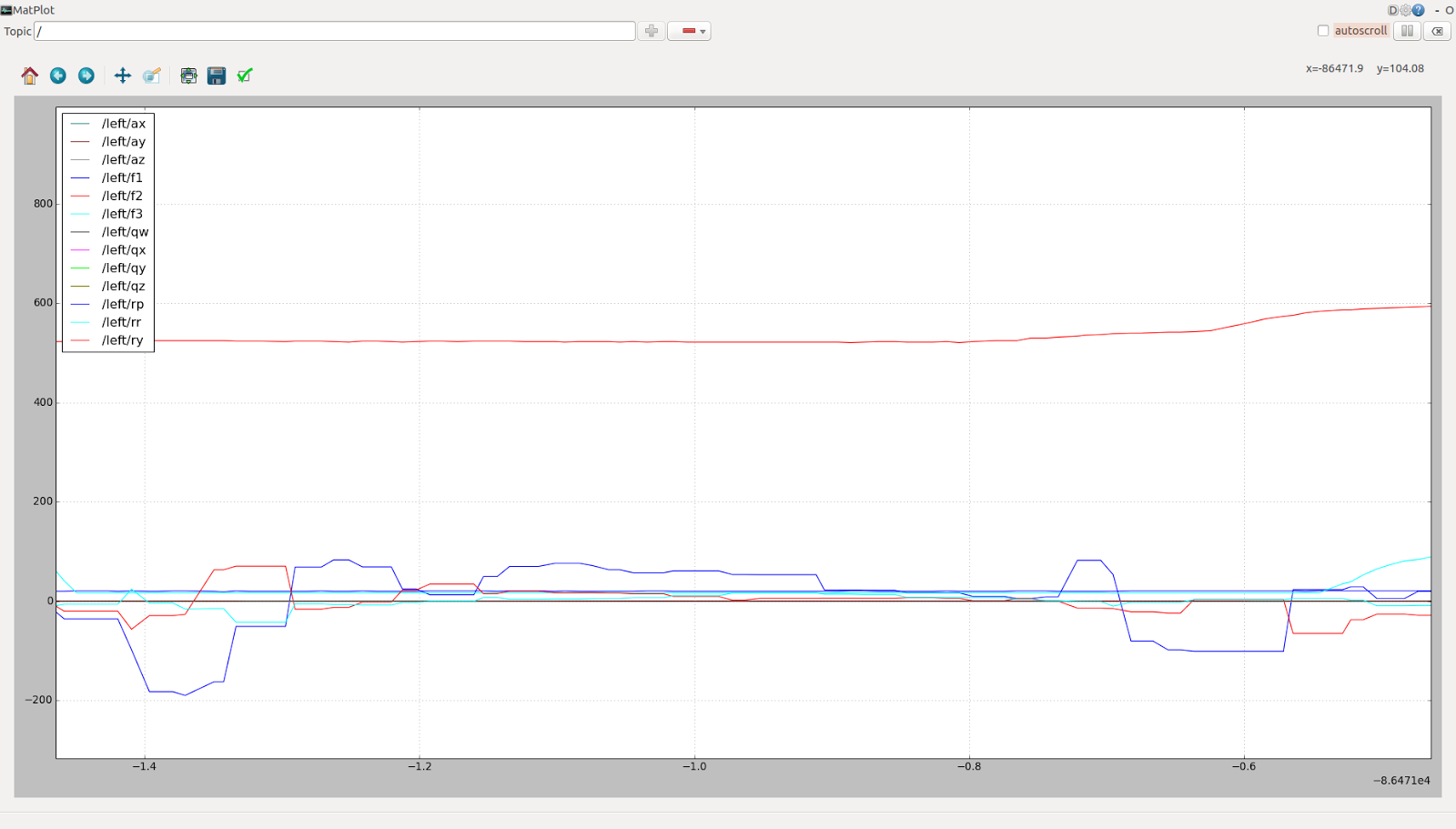
Figure 7: Data acquired by the family of on-board sensors from the treadmill experiment

 

Each of the main sensing components has been interfaced with an Arduino Mega, and a ROS-Arduino interface has been set up using nodes and ROSSerial. The sensed data can be viewed in the terminal itself by echoing the topic corresponding to the left or right skate, which makes debugging easier. This data can also be stored in a .rosbag or visualized using rqt_plot and rviz (for the Kinect and IMU). The sensor data is communicated in the form of a customized sensor message in ROS with a single timestamp. This sensor message was mapped to the Arduino library since the publishing node is in Arduino.

The Kinect has been used to generate the user’s centre of mass, as seen in Figure 8 (below), and x- and y-axis displacement (horizontal axes) values in meters. The IMU can be used to record acceleration and quaternion data as well as gyroscope data for orientation of the foot. The acceleration data can be integrated to get velocity and positon; however, currently the integrated output is too noisy to be of any consequence. The force sensors have been mounted and connected to an analog pre-processing circuit which works as a differential amplifier with a high input impedance and provides a satisfactory resolution over a large range of forces. There are three force sensors per skate; two under the ball of the foot and one under the heel. This configuration was selected in order to get the maximum possible data that may be useful even for omnidirectional movement with as few force sensors as possible. The optical encoders (one for each driven wheel) are used in the position and velocity control loops as a feedback. The encoders are used to give us the angular displacement, and in turn the position in digital form. The treadmill experiment (data visualised in Figure 7) served as a major validation for the sensing subsystem and allowed us to test our integrated system in a controlled environment.

 

  

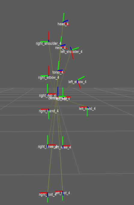
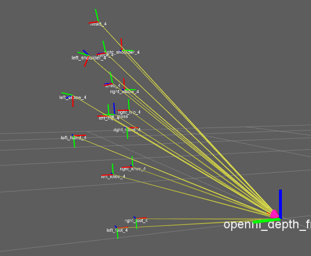
Figure 8: Centre of mass estimation using the Kinect

Testing for this subsystem was carried out initially at a component level; with each sensor being tested individually and then, as each new sensor was integrated, the subsystem was tested again. When testing individually, the Kinect provided reasonably accurate values for distance and for centre of mass, as mentioned previously. Each force sensor was tested with forces that were small at first but grew increasingly large until the output saturated.

 

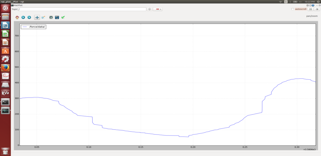
Figure 9: Force plot for a single force sensor

 

Each of the encoders were tested individually, then as a pair corresponding to one skate and finally for the pair of skates. The inertial measurement units were tested initially for direct communication with the laptop but had to be reconfigured to communicate with Arduino at a desired baud rate and frequency.

The sensing subsystem made use of two routines; the Kinect zero-point routine to calibrate and test the Kinect, and the force sensor calibration routine to calibrate for a user’s weight. Data is sensed at two frequencies; 30 Hz (by the Kinect) and 100 Hz (by all the other sensors).

As previously mentioned, the treadmill experiment played a very big part in the validation of the sensing subsystem. It can be seen from the two sets of force plots depicted in Figure 10 (below) that the force profile is periodic and tends to saturate at the peaks in the vertical direction. These force profiles are also verified by the theoretical walking z-force profiles observed in biomechanics. The IMU data collected is a little noisy as we can see from Figure 11, likely because of impact.

 

   

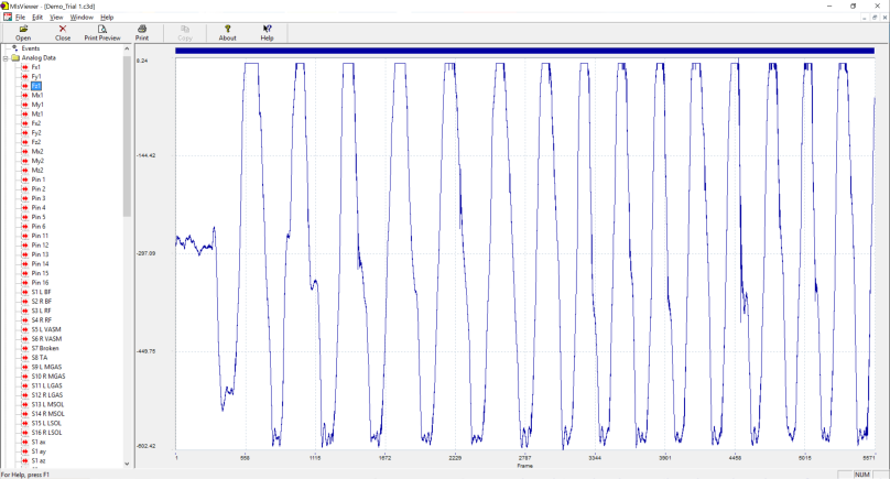
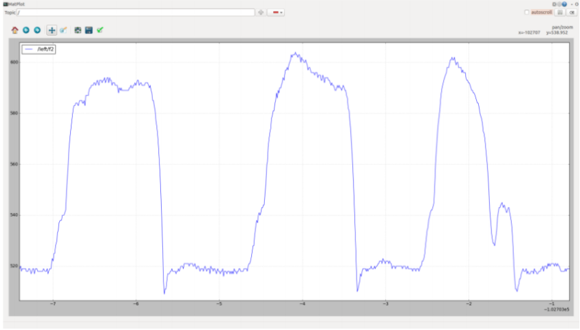
Figure 10: Comparative force plots from treadmill experiment; Skates (left), and Treadmill (right)

   

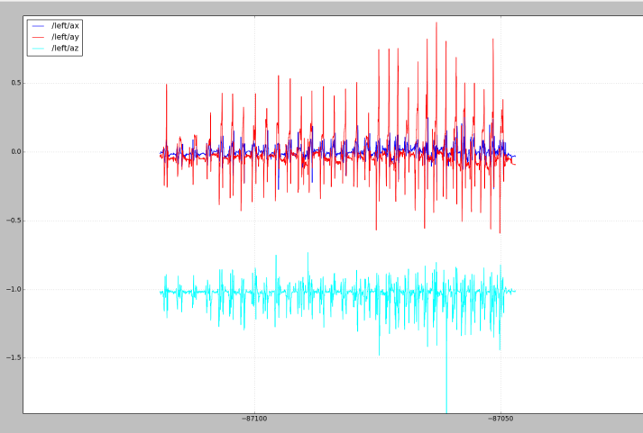
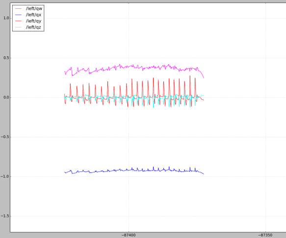
Figure 11: IMU plots from treadmill experiment; Quaternions (left), and Acceleration (right)

The encoders played a large role in the controls subsystem, but were not a part of the treadmill experiment.

II. CONTROLS

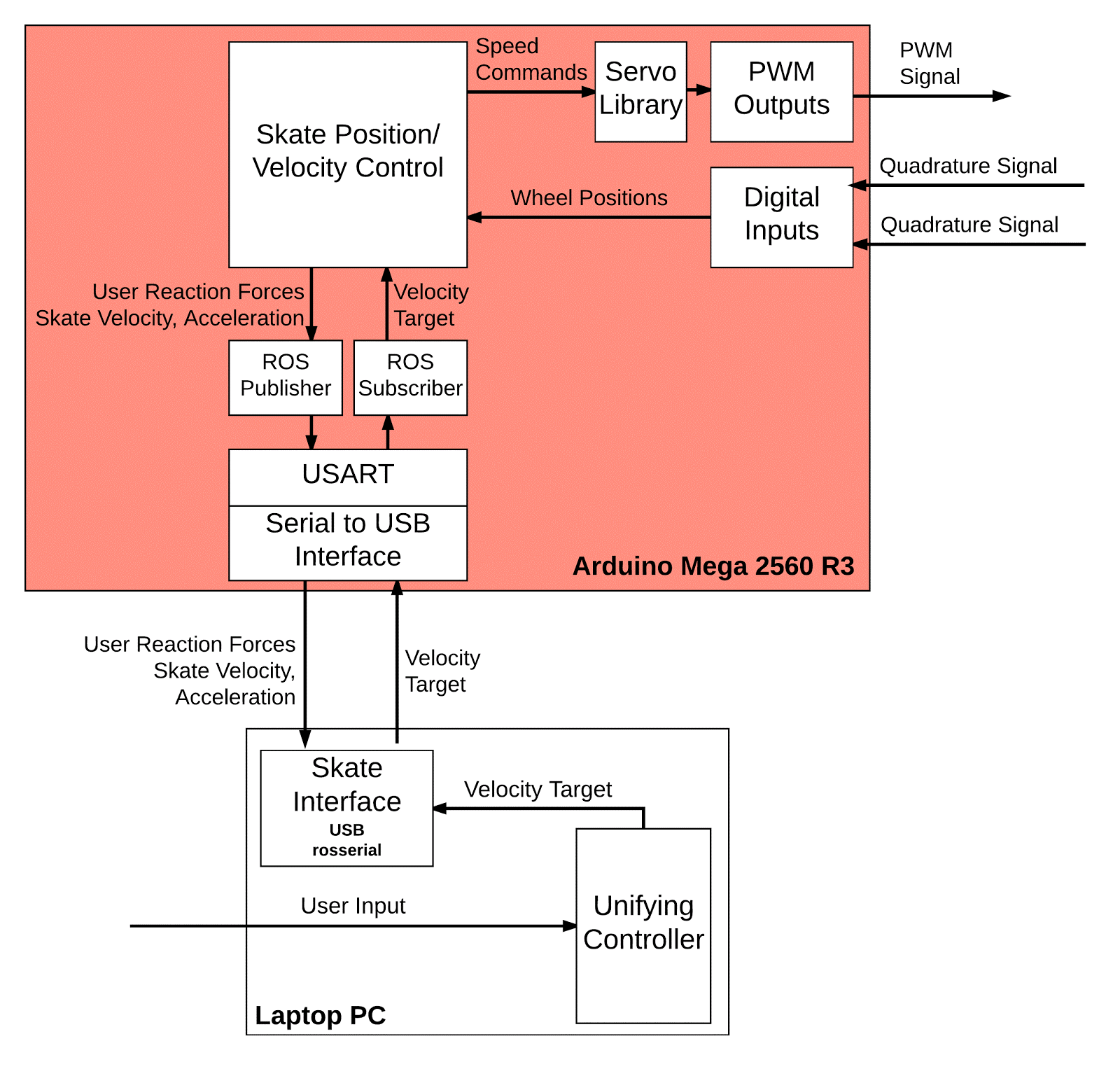
Figure 12: Cyberphysical architecture – Controls focus

Figure 12 (above) illustrates the controls aspects of the Cyberphysical Architecture that were implemented in the Fall Semester. A keyboard input ROS node allows the user to designate a target velocity, which is communicated to each Arduino via a matching rosserial node, and then controlled to at each skate. At Arduino power up, the code waits for data to be published on subscribed ROS topics before configuring outputs and interrupts, thereby keeping the skates in a safe state until user control is available. In addition to the progress in developing the communication and process infrastructure in ROS, the majority of the control focus was in the development of the Skate Position/Velocity Control that culminated in Arduino code executing on each powered skate.

One position controller and one velocity controller was implemented per motor. The position and velocity value is currently determined by one optical encoder per wheel, which is tied to the Arduino’s external interrupt pins. When the external interrupt is triggered for a given channel of an encoder, the associated interrupt service routine is called to update a counter. This counter is converted to an absolute position using the pulses per revolution rating of the encoder, the diameter of the wheel, and the circumference formula. This position is then filtered using a four-sample moving average filter at 1 kHz. From this filtered position, a rough velocity is calculated using the difference of adjacent samples at the sampling period. This velocity calculation is also filtered using a four-sample moving average filter at 1 kHz.

A state machine is used to determine which controller to run; the state machine and controllers are executed at 250 Hz. (Fixed) Position control is the default state. In this mode, the controller provides motor speed commands which are proportional to the error between the current location and the target location. In order to circumvent the one second delay imposed when reversing command direction to the speed controllers, the front wheel resists only forward motion while the back wheel resists only backward motion. When the target is updated to a non-zero value, the state machine transitions from position to velocity control; during the transition, the encoder counts and all of the controller sum/integral terms are intentionally reset. In this mode, the controller provides motor speed commands which are proportional to the sum of the differences between the current velocity and the target velocity over time. To ensure user safety and comfort, an acceleration limit is imposed on the target velocity to facilitate ramping between position control and a goal velocity. Lastly, the system transitions back to position control if the target velocity is zero and the acceleration limited target velocity is less than 20 mm/s; once more encoder counts and error sums are cleared.

Speed commands are issued to the electronic speed controllers as pulse width modulation (PWM) output. The output waveform is generated using the Arduino servo library with a modification to increase the waveform update rate from 50 Hz to 250 Hz to align with the controller execution frequency. The built-in mapping function is used to circumvent the controller dead band by remapping -100 to 0 speed commands to pulse on-times of 1,000 to 1,480 microseconds and 0 to 100 speed commands to on-times of 1,520 to 2,000 microseconds.

A layered approach was used for system testing and validation after each major update. The skates are placed upside-down on the benchtop and powered on. Position control is verified by disturbing each wheel in the controlled direction. Velocity control is verified by commanding various velocities and comparing the target to the achieved results. Depending on a change impact analysis, position and velocity control may be re-verified next on a single foot. At the start of each dual foot test, position control is re-verified, and only then are velocity control tests performed.

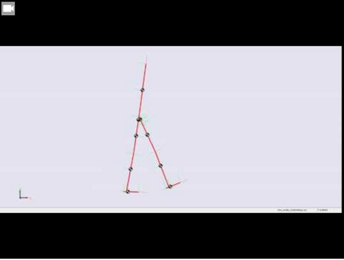
The control system was initially designed and preliminarily validated in Simulink. The validation effort including utilizing Hartmut Geyer’s Neuromusculoskeletal SimMechanics model^[10] and replacing the horizontal ground contact model with a controllable ideal force actuator. By commanding a 1 m/s skate velocity, the model figure remained well-centred with minimal drift, particularly given the open-loop nature of the control. This model, along with data collected during the instrumented treadmill experiment, will serve to validate further controller designs.

During the Fall Validation Experiment, the position controller met and exceeded the success conditions by maintaining fixed position control to within a tighter band than specified throughout all planned motions as well as unplanned disturbances. The velocity controller met the success conditions by effectively achieving the velocity target and exceeded the conditions by doing so for a greater amount of time by nearly a factor of three and within a tighter position band by nearly half.

The strong points are the simplicity, efficacy, and robustness of the implementation given the available time, enabling completion of Fall Validation Experiment activities. The main weak points are somewhat coupled to other components of the design, particularly the reversal issues and poor low speed performance of the off-the-shelf speed controllers, and command stability that can be improved through tuning and traction improvement. The major area of refinement is completion of the controller implementation by integrating the force sensors, Kinect, and inertial measurements units, which will be the main work in the Spring semester.

 Spring ’17

---

One of the first changes implemented in the second phase of our project was to move the PCB stack (which includes the PCB, the Arduino, and the IMU) from under the skates to above the user’s toe-box. This was mainly done for 2 reasons –

1. Eliminating the need for a PCB casing to protect the components from physical damage, hence simplifying the design and preventing the bottom of the skates fro becoming too cluttered
2. Freeing up space under the skates, thereby allowing more space to solve issues like –
   1. Skates halves misaligning
   2. Skates unable to accommodate varying foot orientations
   3. Cable management system

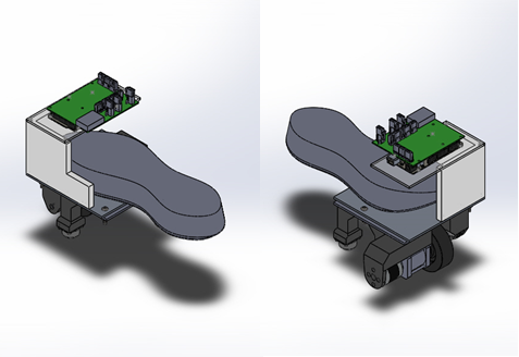Figure 13: CAD rendering of the new PCB stack mount

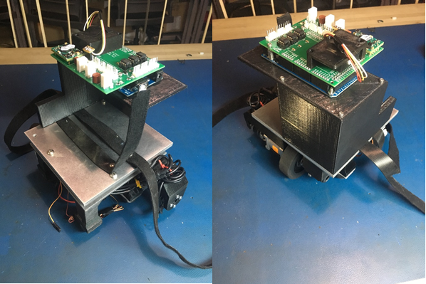
Figure 14: New PCB stack mount assembled on the skates

Due to changes in the PCB, there were further changes made to the mounting plate, with the IMU removed from the stack and placed alongside the Arduino, as shown below.

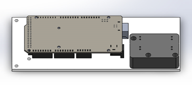
Figure 15: CAD rendering of the next revision of the PCB stack mount

PCB reiteration

The major changes from the previous design include re-wiring the force sensor circuit in order to connect the sensor outputs to the correct pins on the instrumentation amplifier, isolating the motor power from the sensing suite and making digital and analog pin arrays available for use. The ground plane for the sensing suite has been kept isolated from the motor power ground. Previously, the circuit directly connected the grounds of the motor power and the regulator. The speed controllers we are currently using have protection against overcurrent, overvoltage and provide a common ground connection that is indirect rather than the explicit connection we made use of previously. The power regulator was removed due to its operation being intermittent despite it being a commercial, off-the-shelf product. It does not need to be replaced as we can make use of the Arduino Mega’s regulated power out, since the current requirement is well under the maximum of 200 mA the Arduino is rated to supply. We also decided that we need to add indicating pins for each skate, such that we can have a single code running on both skates. I added these and made digital and analog pin arrays (six and three, respectively) available for debugging and development if needed over the remaining semester. A dead-man’s switch has been added as an additional safety feature. The board houses a potentiometer for the third amplifier circuit, which allow us to get a variable gain that can be tuned/altered as required for the rear force sensor. Also, this gives us the freedom of making the gain as close as possible to 1000 without facing the issue of non-linearity in the IC operation.

Spade terminals

Another change implemented on the hardware side of things was the addition of spade terminals to the force sensor wires, which were too fragile by themselves. The other end of the spade terminals were fitted with 22-gauge wires. To prevent vibrations from potentially tugging on the fragile wires, mounts were designed to hold the spade terminals firmly to the bottom of the skates.

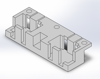
Figure 16: CAD rendering of the spade terminal mount

Force sensor calibration

One of the major challenges was in applying a significant and consistent force to the force sensors in order to determine the mapping between load force and ADC value. Two testing rigs were designed to bolt directly to the top of each skate half in lieu of the top plate that the user stands on. Each testing rig contains a die spring with a known spring constant that is held between a bottom load applying screw and a top load control screw. When the top screw is in the up position, only the weight of the internal hardware is applied to the force sensor. When the top screw is in the tightened down position, a known load is applied based on the spring compression distance, which is fully repeatable by loosening and re-tightening the top screw. By using washers as spacers, and choosing from available screw lengths, the rigs were designed to apply between 110 and 120 pounds of force, which is 55 – 60% of the full range of the primary force sensor.

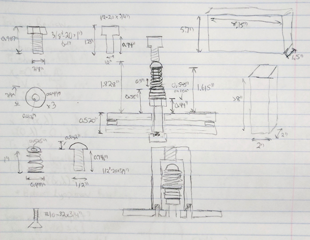
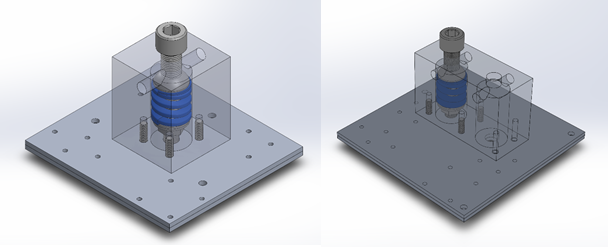
Figure 17: Sketch and CAD rendering of the force calibration rig

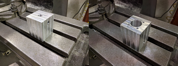
Figure 18: Manufacturing the force calibration rig

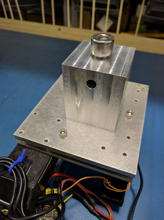
Figure 19: Force calibration rig assembled on the skate

 We decided to correct the preload by the top plates using a software routine. A routine in the code separately calculates the preload that can be subtracted from the weight readings during operation.

The preload must be as low as possible to get the maximum range of the sensors. The routine runs for all the three sensors in one skate. The math going on behind the routine is:

1. The sensor gain: k = (Rl – Rb)/F = Analog/pounds
2. Preload Weight on the sensor Fp = (Rp – Rb)/k = Pounds
3. W = {(R – Rb)/k} – Fp = Weight by user in pounds on the sensor

We first calculate the bias and gains on each sensor. Later calculate the preload after fixing the plates. The threshold to limit the preload on each sensor is 70 pounds. The normalization routine is a service that calculates the total pounds on both the skates when the user stands on the skates while calibrating for the Kinect. The total weight is then used to calculate the percentage body weight on each of the sensors. The gait determination routine is simple for now. It just has thresholds applied on the different force sensors. The thresholds were calculated empirically.

For added range and cable robustness, the rear skate force sensors were replaced with load cells rated to 200kg. In addition to the range difference from the 200lb sensors, the output amplification is significantly less at 1mV/V as compared to 20mV/V. The gains on the instrumentation amplifiers for these sensors was increased conservatively to avoid entering the nonlinear amplification regime. However, the calibrated results from these sensors appeared wildly inaccurate. Further investigation revealed that the sensor outputs did not start changing until after a significant load was applied, violating the fundamental assumption of the gain calibration procedure that assumed a fairly linear progression from unloaded to the test load. Figure 20 illustrates how the deadband reduces the calculated gain as represented by the slope of the diagonal lines. By increasing the in-amp gain, it was possible to eliminate this deadband behavior as shown in Figure 21. This test was performed by placing a skate half on a scale and taking snapshots of the scale and multimeter displays while manually applying increased loads in steps.

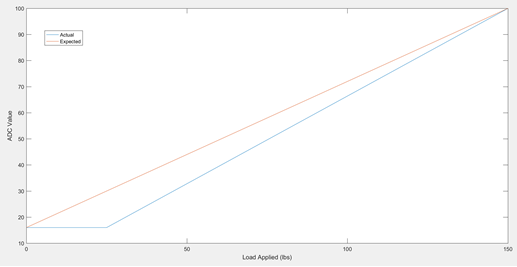
Figure 20: Force Sensor Deadband vs. Gain Calibration Assumption

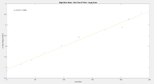
Figure 21: Known Load vs. In-Amp Output Voltage

Object-oriented code refactoring

At the end of the prior semester, our Arduino code base was segmented into encoder-based controls code and inertial and force sensing code, whereas our final adaptive control requires sampling force and inertial data while computing control outputs. However, the control code file was already fairly lengthy and would become potentially unmanageably long after adding the additional sensing code. To improve the readability and maintainability of the code, it was decided to refactor the code from C to object-oriented C++ libraries.  The control code was divided into two classes/libraries: Drive and Control. The Drive class interfaces with the speed controller and encoder on a single drive unit, estimates wheel position and velocity based on the encoder measurements, and updates command to the speed controller. The Control class provides the implementation of the position and velocity controllers and determines the appropriate mode and controller to execute based on system state.  Within the main sketch Skate, two objects of each class were instantiated, one for the front and one for the rear portion of the skate. The main sketch also contains the setup code, the rosserial interface, a sampling loop and control loop, and the interrupt service routines.

State Machine and Sensing

The controls work based on the Kinect offset and the sensing suit’s output. To validate the idea of re-centering, we conducted experiments using Simulink where a walking model was given force on each foot while on ground. Figure 26 represents the simulation.

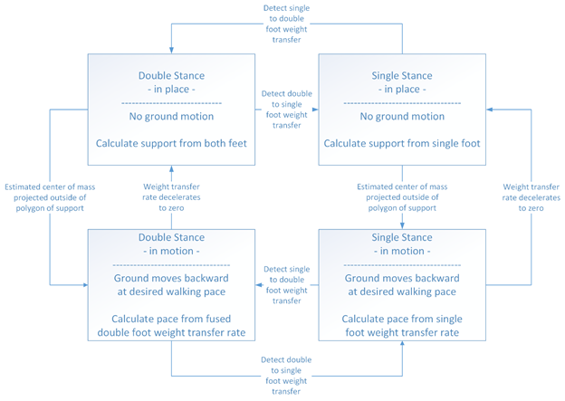
Figure 22: State machine

An object-oriented finite state machine has been implemented in python; currently, it has four states, with transitions between each state and an entry and exit function for each state. The state machine currently takes a user input as a string, and transitions to the required state (or remains in the same state). Each state object also has a ‘stateID’ attribute, which will be useful to integrate this code with the main code and the output received from the SVM. The figure below shows each of the states with their entry and exit functions.

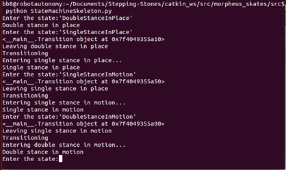
Figure 23: State machine implementation in Python

Figure 24:  Kinect User tracking

 

 

 

 

 

 

 

                                                                       Figure 25: Skate based sensing output

The tests tried to capture as much variance as possible in both the test cases. We also kept trying to change the pre-load between the tests so that we can add that run time noise to the data. We tried to fit this data using different models like stochastic gradient descent, linear SVM and RBF-SVM. Among the three types, we could learn well using the RBF kernel SVM. The performance seems promising with respect to execution time, training time and accuracy. The accuracy should be credited to the visibly separate clusters from the force sensors.

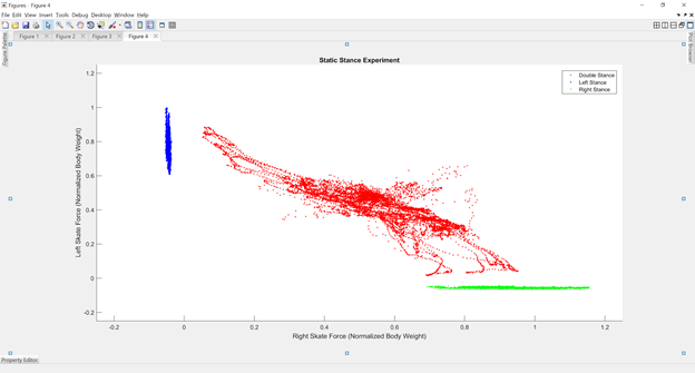
Figure 27: Clustering the force data from static experiments

Software architecture:

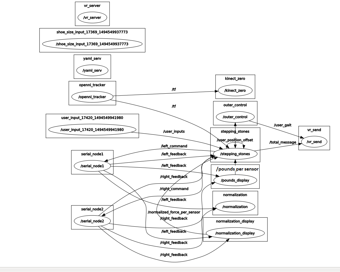
Figure 28: Rqt_graph of the software Architecture

The software architecture is designed around ROS. Figure 28 displays the rqt_graph of the whole software running. The higher level control is written in the user_gait that runs the state machine and stepping stones sends the command targets along with Kinect data processing.

Virtual Reality

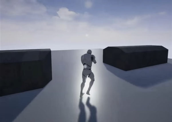
Figure 29: Demo virtual environment

We tried 3 main approaches to completing the communication pipeline from the ROS Master to the VR game engine. These were –

1. Trying to integrate the websocket script implemented last week with the script that enabled Unity to import a DLL and access functions from it.
2. Writing the data received from the ROS Master into a file in Windows, and simultaneously reading from the file in Unity.
3. Classifying the message received from the ROS Master into one of five-speed modes, and simulating a distinct keystroke for each of these modes, while designing the game to react appropriately to these keystrokes.

The last approach was most successful among the 3. We decided to switch over from Unity to Unreal Engine (UE) as our choice for the game engine to work with, for 2 reasons –

1. Designing game content from scratch is a lot more intuitive in UE than it is in Unity, mainly due to the “Blueprint” feature available to work with.
2. The team received a game (Robo Recall) along with the purchase of the Oculus Rift, and it is open source. It can be “modded” using UE. Time and scope permitting, we would like to modify the game to interface with the skates.

Exporting the websocket script into a DLL, and accessing from Unity

This was the first of the three approaches we tried in completing the communication pipeline from the ROS Master to the VR game engine. The problem we were facing was to come up with a method to allow Unity to access the data coming in from the ROS Master into Windows.

Unity has a feature that allows it to import DLLs, and access functions from within it. We started off by writing a simple C++ function that takes an integer as an input, increments it by 1, and returns the new value. We built this function into a DLL file on Visual Studio, and followed the appropriate steps to import it into Unity. From Unity, we could pass an integer into this function and get back an appropriate value.

Since this seemed promising, we proceeded to try and convert the script that enabled communication between the ROS Master and Windows into a function that can be exported to a DLL. Even though we managed to make a DLL from it after numerous attempts at fixing bugs, running the function from within Unity did not facilitate communication with the ROS Master. Since the framework for this script was taken off the ROS Wiki, we didn’t have a deeper understanding of it to realize what needed to be done to fix this issue. Hence, we decided to change my approach to this problem.

 Writing data into a file, and reading it from Unity

The second approach we tried was to write the data coming in from the ROS Master into a file in Windows, and simultaneously read from the same file in Unity. This idea had occured to me earlier, but we wanted to avoid trying this method as far as possible, since we have had bad experiences with simultaneous file write and read operations.

This approach did manage to complete the communication pipeline. However, as expected, the performance was quite unreliable. Since the file needed to be closed and re-opened between each write operation, we suspect it was contributing a lot to the latency. The communication from the ROS Master to Windows is designed to not lose any messages, and to do that, it queues up messages it received while the previous one is still being processed. However, there is a limit to this queue size beyond which it terminates the program. When trying to write into a file, the program always terminated after a few minutes of use.

Moreover, due to reasons we still do not fully understand, the messages would be written into  the file in “batches”, with a large delay after each “batch”. Due to the unreliability of this process, even though it was working to some extent, we decided to explore further options.

Simulating keystrokes

We got this idea from reminiscing my undergrad days, when some students would write scripts to simulate rapid keystrokes (much faster than possible by a human) to beat certain computer games. The code for doing the above is quite simple, and integrating this into the communication program didn’t prove too difficult.

The idea was then to classify the data coming in from the ROS Master into speed modes (very slow, slow, normal, etc.) and have distinct keys assigned to each of these modes. Then, depending on the mode that is activated by the message at any instant in time, that keystroke can be simulated. This approach worked out very well, with no detectable loss in data.

Designing the VR game

The next step was to design VR content on which the above communication pipeline could be tested. As we mentioned above, we decided to move forward with Unreal Engine instead of Unity because of its intuitive blueprint feature, and the possibility to expand to a full-fledged game for SVE.

Even though blueprints made this task easier, it took us a while to familiarize ourselves with the architecture and features of UE. Once we began to feel comfortable, we started to design the character and the camera movement using the Animation Starter pack available online for free. This pack allowed us to use ready-made human models and animations, and let us focus more on the camera translation and logic flow. We designed two games – the first with the camera behind and above the character, resulting in a 3^rd person perspective (pictured above); and the second was a 1^st person view of the world.