The processing subsystem includes all algorithms within the system, including: signal filtering
and conditioning algorithms, prediction and calculation algorithms, and the control algorithm. It
will take raw sensor data as an input into the subsystem and output torque values to the actuation
subsystem.
20thJanuary 2019
An Initial Git Repository was set up in order to facilitate version control and code updates.
7stFebruary 2019
Research Completed on on-board computers for the project. NVIDIA jetson was chosen. Sparkfun Razor IMU 9 Dof was picked out, to be placed at knee to collect walking data.
16thFebruary 2019
Sparkfun IMU was interfaced with Arduino Uno (I2C protocol). FSR’s were connected to analog port of Arduino. The IMU’s firmware was modified to give roll, pitch, yaw and quaternion values along with accelerometer, gyroscope and magnetometer values. The FSR’s data is intended to provide ground truth for the prediction model.
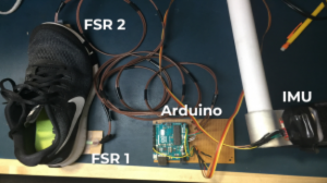
Fig 1: FSR and IMU setup with Arduino
20thFebruary 2019
Preliminary data collection was done with the setup for one of the team members. The values were read from the Serial monitor of the Arduino IDE through a python library. The data collected was then converted to a pandas Dataframe to do exploratory analysis.
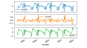
Fig 2: Accelerometer Values from IMU
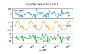
Fig 3: Gyroscope Values from IMU
7stMarch 2019
Additional data was collected with the IMU on the brace fitted at the front and properly calibrated. The analog values from FSR were binned and binarized them (as shown in the figure below), by noting the values from the start of a heel strike till a toe-off. A threshold of 400 was set and binarized the values at the heel and toe.

Fig 4: Binned FSR values
In the above diagram, for the purpose of clarity, the values at stance have been assigned 500 and values at swing have been assigned 0. For the purpose of training a model, we assigned 1 to the values in swing and 0 to the values in stance. This is added as the last two values of the data frame. Then we implemented a vanilla logistic regression on the model and performed a 10-fold cross-validation.
The cross-validation accuracy was about 95%
Then we prepared a different dataset altogether (completely exclusive from the training data) and fit the trained model to that. We were able to obtain a accuracy of 81%.

Fig 5: Test data vs Predicted Data

Fig 6: ROC Curve for Logistic Regression
Understandably so, the model provides the prediction at that specific data point or instant independent of previous values.
13thMarch 2019
Foot Placement: For the Foot -placement section of the Processing Subsystem, we researched on the various models and chose the Linear Inverted Pendulum Model to calculate capture point.
22ndMarch 2019
A Preliminary Software Architecture pipeline was drawn up with our initial understanding and flow of all the algorithms.
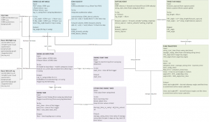
Fig7: Software Architecture
1stApril
An initial ROS Environment was setup including the required packages for the YOST IMU and Razor IMU on Git.
The Firmware on the Razor IMU was modified to read the FSR values. This is to remove the Arduino from the Pipeline and directly interface FSR to the IMU (SAMD21 Breakout Board) to the Jetson.
The FSR and resistors (for the voltage divider circuit) were soldered to the perfboard, in order to collect data.
5th April
ROS Environment:
The Figure below shows the ROS architecture currently implemented for the exoskeleton system. The Razor IMUs ROS package allows for the linear acceleration, angular velocity, and roll, pitch, and yaw angles to be published. For testing and validation purposes we also set them to publish the raw FSR values to determine ground truth of whether the leg is in stance or swing (The FSRs are directly connected to the IMU breakout boards). This data is published to the /imuR topic for the right leg and the /imuL topic for the left leg. The classification_model_node, COM_vel_cal_node and hip_exo node all subscribe to this topic. The classification_model_node determines if each leg is in swing or stance and publishes this information to the /swingLegRight or /swingLegLeft topic for the right and left legs respectively. The COM_vel_cal_node and hip_exo node subscribe to these topics. The COM_vel_cal_node calculates the CoM velocity and publishes it to the /COM_vel topic. The hip_exo node subscribes to this topic. Within the hip_exo node, the capture point is calculated and then transformed into a desired hip angle for the leg in swing. The HFE and HAA desired angles are published to the /desiredAngleR or /desiredAngleL topic, depending on which leg is in swing. The motor controller node will subscribe to these topics so that it can actuate the motors at the hip joints appropriately.
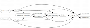
Fig 8: ROS Architecture
7th April
Logistic Regression and the Random Forest Classifiers are the two machine learning models were considered for swing leg detection. The nine features from the IMU (linear acceleration in x,y,z, angular velocity in x,y,z and roll pitch and yaw) are normalized before being used as inputs to the models.
The data was split into training and testing sets. The two models were trained on the normalized dataset of IMU values and the target class. The cost of false positives is quite high for the exoskeleton use case. A false positive is when the leg is in-stance but detected to be in-swing. This would lead to the stance leg being actuated further in the software pipeline, which is potentially dangerous to the user.
The confusion matrices for both logistic regression (Table 1) and random forest (Table 2) are as following. We achieved 94% overall accuracy for logistic regression and 97% for random forests.
Table 1: Logistic Regression Confusion Matrix
| Logistic Regression | Predicted Leg in Stance | Predicted Leg in Swing |
| Actual Leg in Stance | 822 (TP) | 53 (FP) |
| Actual Leg in Swing | 58 (FN) | 943 (TN) |
Table 2: Random Forests Confusion Matrix
| Random Forests
(50 estimators) |
Predicted Leg in Stance | Predicted Leg in Swing |
| Actual Leg in Stance | 870 (TP) | 5 (FP) |
| Actual Leg in Swing | 57 (FN) | 944 (TN) |
It was concluded that the Random Forest Classifier with tuned hyperparameters provided the least number of false positives. Hence this classifier was used for the final system. Precision and recall within the range of 93-99% were obtained for the final spring validation demonstration.
The subsystem should be improved by the decreasing the algorithm processing time to 100ms. It would also be beneficial to smooth the predictions by taking into account the temporal nature of the data and noting the change or transitions in IMU values from swing to stance.
10th April
CoM Velocity Calculation:
The CoM velocity calculation subsystem takes the roll and pitch angles from the thigh IMUs as well as predicted swing leg as inputs, and calculates the human’s center of mass velocity which is used for the prediction of the capture points. We use the stance leg as an inverted pendulum model as shown in Figure 18. Using a series of inputs of IMU angles and time stamps, we calculate the angular velocity. With a fixed length of human’s leg, we can calculate the linear velocity of the end the pendulum, which can be regarded as human’s CoM velocity.
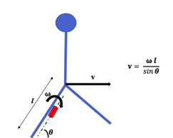
Figure 18: Inverted Pendulum Model for CoM Velocity Calculation
Since the CoM Velocity calculation depends heavily on the correct detections of the Swing Leg Classification Subsystem, we first tested with the ground truth swing and stance leg values obtained from the FSRs under the feet. We started with sampling the IMU angles continuously and used the differences of angles divided by the time intervals to get the angular velocity. However, since the time intervals for continuous sampling is too short, a small difference caused by noise will result in large calculated velocity. To mitigate the influence of noise, we improved the sampling intervals. Also, we use the average of the calculated velocities at 10 different samples as our output velocity to further mitigate abnormal values.
September 12 – Oct 1st ,2019
Time profiling of the software pipeline was done as shown in the. Figure below. The entire software pipeline was also revamped and three major packages were created: soteria sensing, Soteria controls and soteria motor control.

Figure 19: time profile of pipeline
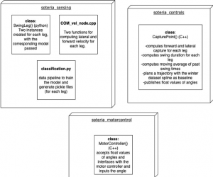
Figure 20: software pipeline revamp
September 28, 2019
Came up with the winter dataset based trajectory planner concept. Sourced an excel version of the winter dataset and extracted the required columns for the trajectory planner.
October 22, 2019
Began implementation of the winter trajectory planner in MATLAB . Wrote code in MATLAB to read data from the excel (.csv) file and import it into MATLAB as array objects. Thresholded the ground reaction force column and plotted it alongside the HFE curve to identify the swing phase and stance phase. Figure 1 shows one complete gait cycle along with a thresholded GRF plot.
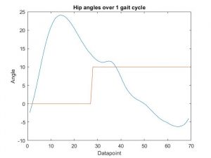
Figure 1: One complete HFE trajectory cycle with the thresholder GRF plot denoting swing and stance
October 23, 2019
Extracted the section of the trajectory over swing, and divided the datapoints by the last swing-phase datapoint so as to normalize the trajectory to end at unity. The normalized swing portion of the winter trajectory can be seen in figure 2 below:
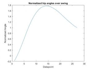
Figure 2: Normalized swing portion of the winter trajectory
November 5, 2019
Ported the normalized winter trajectory from MATLAB to the soteria_controls package in C++. Wrote code to obtain the desired landing angle and swing times from the helper functions. Wrote code to scale the trajectory along the y-axis to match the desired angles, and imported and used the cubic spline interpolation library to interpolate the trajectory in order to scale it by the estimated swing time along the x-axis.
November 20, 2019
Wrote alternative trajectory planner which only follows the rising portion of the curve to the desired hip angle instead of the complete rise and fall. Tested it on the user and determined it to be ill-suited to the problem. Implemented a phase shifter for the trajectory so that the trajectory can act earlier and actuate the leg linkage faster to minimize response time.