Latest updates
Below is the video from our latest field test 5 (03 30, 2016).
https://youtu.be/l0hPuPsgvXc
Below is the video from our field test 3 (Feb 03, 2016).
https://youtu.be/dA29YThXDvg
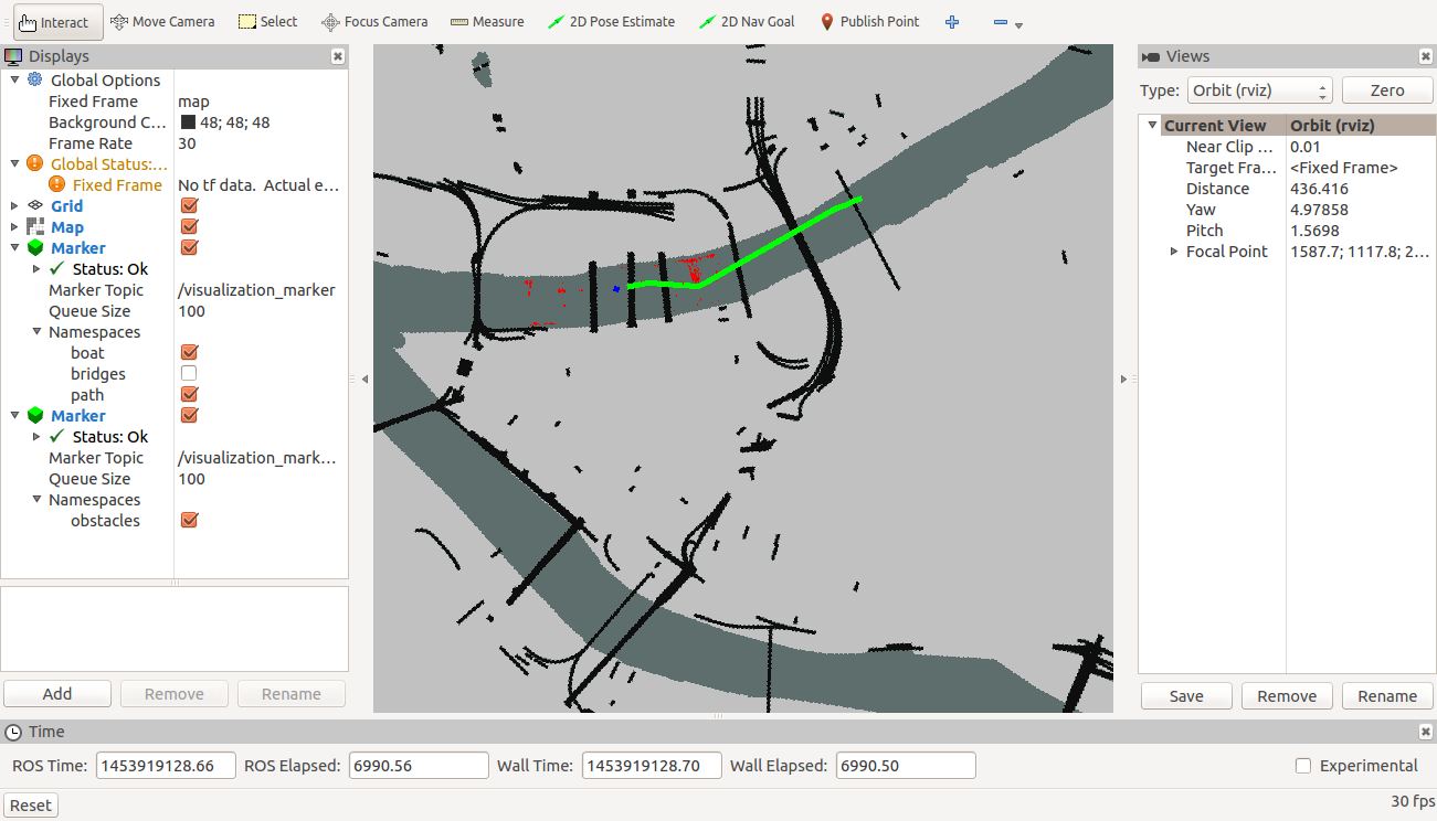
At present, we are able to click the goal location on the map displayed on the Operator Control Unit. Path planning algorithm then uses this goal location to plan the path and directs the low level controlled (by sending way-points) to steer the boat to the goal. This has been tested during our field test conducted on Feb 03,2016. We would be integrating the radar data soon and would be also testing that during our next field Test. The figure 0 below, shows the snap shot of OCU which depicts the current location of the boat (blue color), obstacles captured from radar data (red color) and the planned path (in green color).
Also, for details regarding perception and path planning sub systems see the information provided below:
Summary of the progress that we have made in perception and path planning sub-systems
1. Perception Sub-system
Gathering radar data and segmenting the types of obstacles
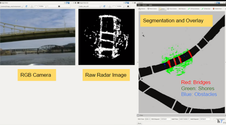
Our first challenge in the perception subsystem was to get data from the radar. No one at NREC had used this radar before so we were unsure how difficult the interfacing of radar would be. We found an open source library OpenCPN through which we were able to collect data from radar. We integrated this with ROS as our entire software architecture of perception and path planning is based on ROS. Next, during the field tests we used an RGB camera in addition to the radar sensor to capture the ground truth. Figure 1 shows collected RGB camera and raw radar data. Our next step was to segment brides, shores and obstacles on the river. We did that by comparing it with original occupancy grid map (with bridges). The output is shown in the rightmost visualization of Figure 1. Here shores are represented by green, bridges by red and obstacles by blue.
Filtering raw radar data
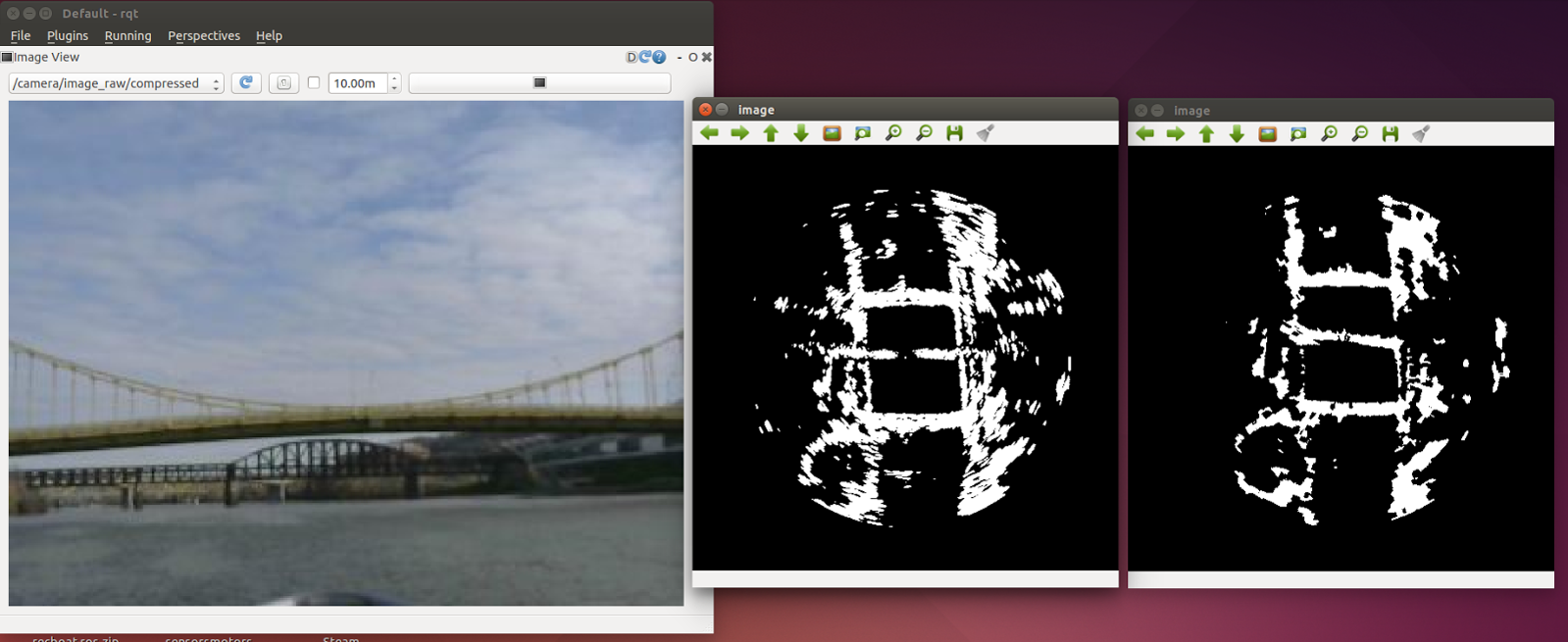
Raw radar data has some false positives which are required to be filtered in order to get correct location of the obstacles. We used a binomial probabilistic filter to get rid of the false positives. Figure 2 shows the result after we apply filters to the data. The center visualization in Figure 2 shows raw radar data and right image shows filtered radar data. We can see that a lot of the false positives are not present in the filtered radar data.
Putting bounding boxes around the obstacles
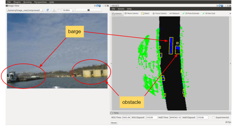
In order to measure the accuracy of detecting obstacles, we need to quantify how many obstacles we are able to detect from the given obstacles in the path. For that, we create boundary boxes around the obstacles. This can be seen from figure 3 which shows bounding boxes around the blue blobs, which are the obstacles. Two of the big obstacles are marked in Figure 3. One of them is a big barge.
Below is the video of recorded raw radar data and its processed output.
https://www.youtube.com/watch?v=m-Rb-1jFTsc
2. Path-Planning and Simulator Sub-system
Occupancy Grid Map
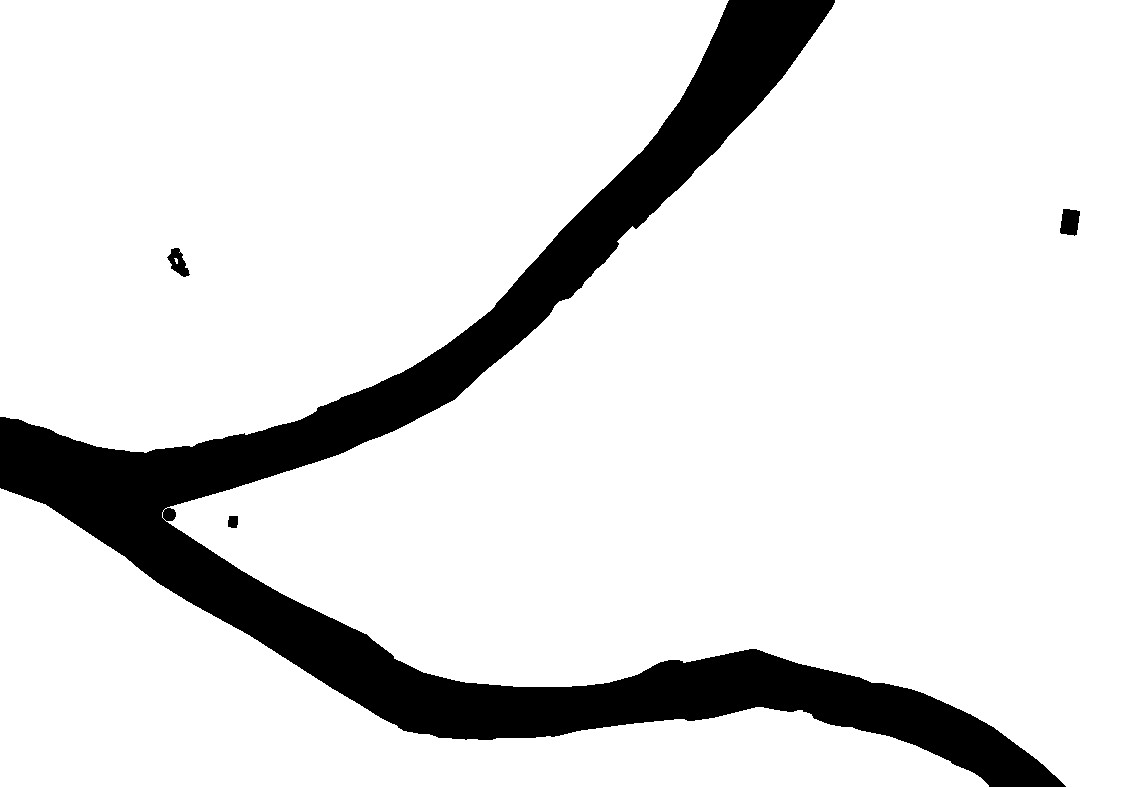
We have created an occupancy grid map (OGM) which the path planning algorithm would be using to find the shortest path between our start position and the desired location. We used qGIS software and openstreet map to extract our area of interest i.e. the three rivers owing through Pittsburgh. Figure 4 below shows OGM where black (zero value of pixels) represents empty path and white (one value of pixels) represent obstacles. The resolution of the map is approximately 5 m.
Inflating the cost near shores and obstacles in Occupancy Grid Map
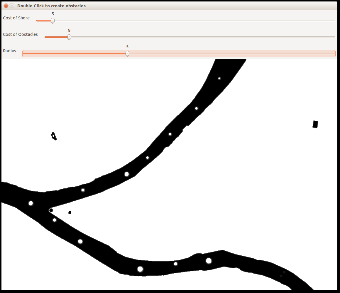
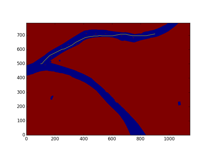
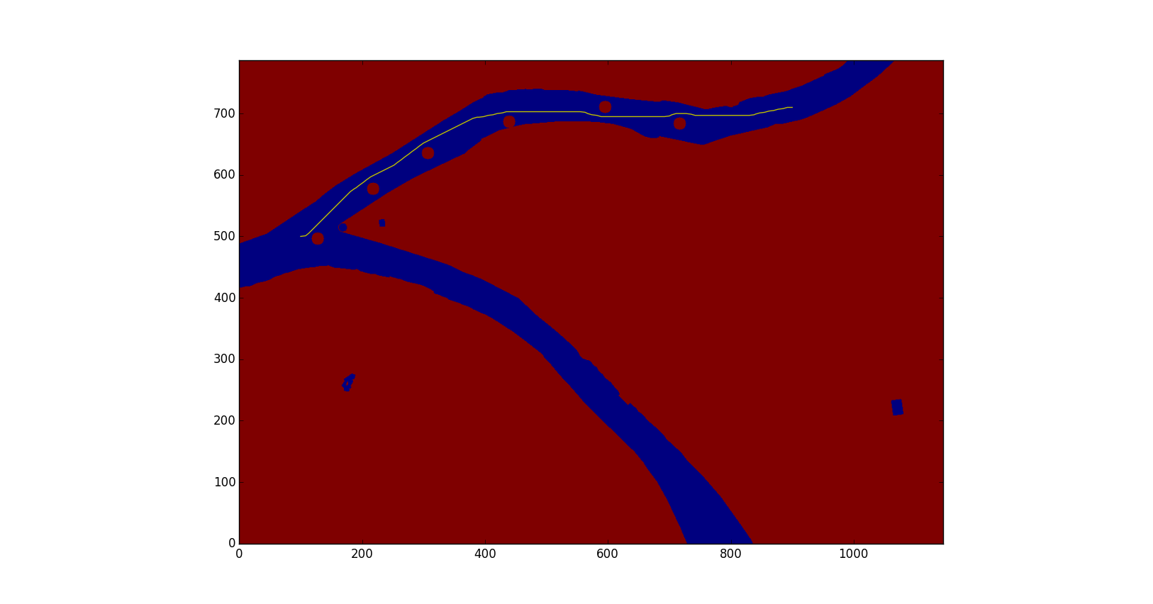
The path planner algorithm tends to nd shortest possible path between start and the goal locations. However, the path generated touches the shores or is very close to obstacles. To overcome this issue we need to inflate the cost (value of pixels) near the shores and the obstacles. We have created a tool which allows us to experiment with modifying these costs through a simple GUI (shown in figure 5). Also, this GUI enables us to add obstacles which we can use to test our algorithms. Figure 6 shows addition of obstacles to the image and the inflated costs (in grey) near shores and obstacles.

Path Planning Algorithms
We are using the SBPL library for planning the path. The library has built in planners like ARA* and AD* algorithms. We converted the OGM to SBPL compatible format and ran the ARA* planner by providing the start and desired location. The algorithms were tested on small, medium and large size obstacles and the visualization of the results are represented in Figure 7, 8 and 9 respectively.

Simulator
As we have limited trials and it takes time for us to test the software on the boat, we needed a simulator to visualize the result of our algorithms. So, we created a simple simulator on RViz where we subscribe to the data given from the path planner, the current location (span pose), and the map server. Figure 10 shows the visualization.
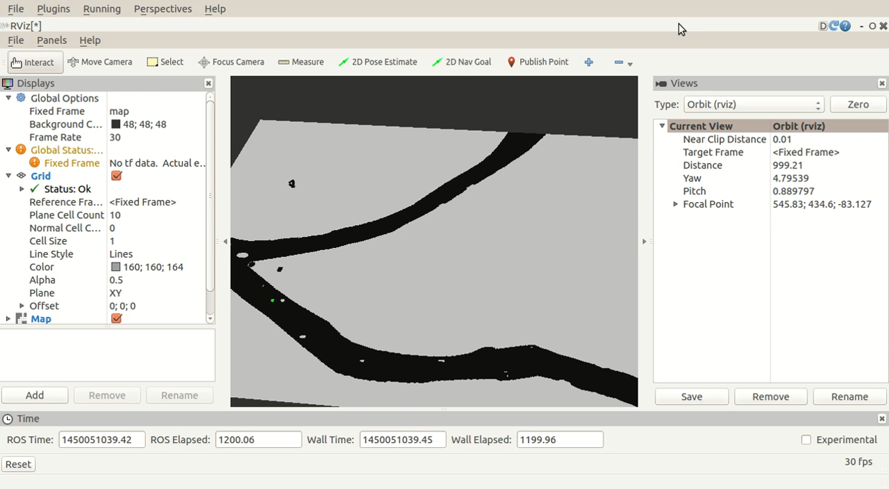
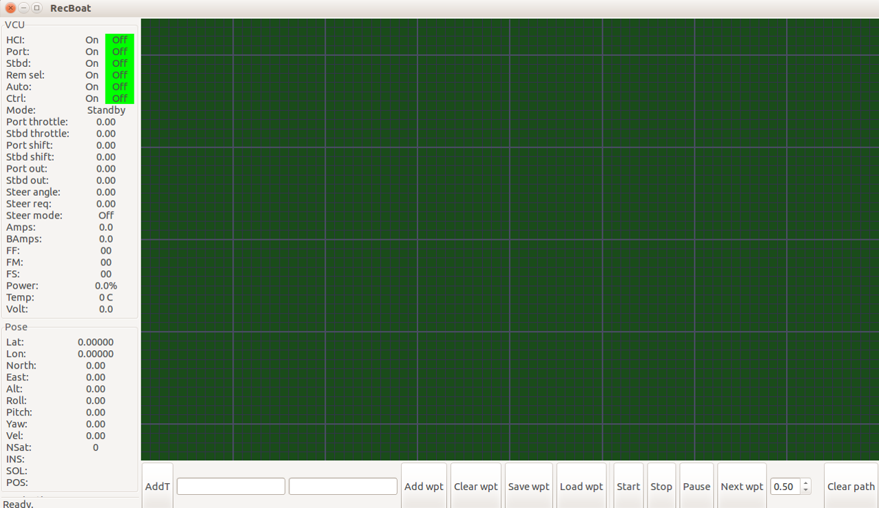
Added features to Graphical User Interface (GUI)
NREC provided us with the GUI which interfaces to the boat. But it didn’t have a feature to add UTM coordinates to the list of waypoints to be navigated. We added this feature in the GUI which can be seen in the bottom left part of the GUI.(shown as figure 11)
Below is the video of the simulator developed using RViz.
https://www.youtube.com/watch?v=6l4n-2rlWy4
3. Printed Circuit Board
There would be some cases (especially in the initial phase of development) where our perception algorithm will fail to detect the obstacles or our path planning will fall to avoid the obstacles. In these cases, if the users of the boat (right now the development team) fail to notice the obstacle (like if they are distracted) then the boat can collide with the obstacle. This can cause heavy damage to the boat or the obstacles. So, to prevent this we need a visualization other than simulator running on our laptop to tell us if the obstacle data is near. This will help us in debugging our algorithms to certain extent.
Solution
We are designing a device called ‘AlertPirates’ which is essentially a new visualization/alarm system of our autonomous water taxi. The system will indicate when obstacles are near to the boat using red LED and a sound alarm. If there are no obstacles in the range of boat then it will show the status with green LED.
The device would be receiving data of obstacles from the perception algorithm running on the laptop. This circuit would be built using ATMEGA 328 microcontroller with Arduino bootloader which will receive serial commands from ROS (ROS topic will publish obstacle presence for Arduino).
Below is the video of the first test run of the PCB. Click here to download schematics and design files of the PCB.