Software System

This page describes the Computing and Software stack that we have implemented to enable to complete our mission successfully.

Robot Operating System (ROS) [12/01/2018]

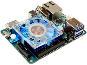
One of the earliest decisions we made was to identify the base operating system and software our robots will be working off of. The computers onboard our two rovers are Odroids XU4s (https://www.hardkernel.com/shop/odroid-xu4-special-price/). They are single board computers powered by ARM running Ubuntu 14.04 LTS. With this computing power it is imperative for us to have an independent computing on both rovers with high fidelity communication capabilities.

For this purpose, we have chosen to use the Robot Operating System (ROS) framework on both our rover which will act as a meta-operating system for your robot. It provides services that one expects from an operating system, including hardware abstraction, low-level device control, implementation of commonly-used functionality, message-passing between processes, and package management.

Both the Odroid computers of the rovers are connected to the WiFi and are communicating to each other and the base station computer. The base station computer acts as the roscore. All the sensors are connected to the computer using USB connections.

 

Range and Bearing estimation as a service [03/03/2019]

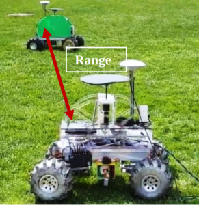
Our co-localization algorithm relies on relative rover information: range and bearing between the two rovers to improve on the localization estimates from the odometery obtained from the encoders and the IMU. To efficiently compute the range and bearing only at the instances where these are required, two services have been broadcasted:

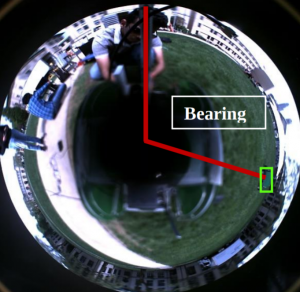
Bearing Service

This service is tasked with finding the bearing of the other rover with respect to the first one. We aim to accomplish this with vision. As per our field experiment, we had decided to use a camera with a catadoptric mirror system to perceive the other rover. The bearing service is subscribed to the image topic from this camera. As soon as it receives a request for bearing of the other rover, it picks up the latest image and performs rover detection, centroid identification and bearing estimation on the image. It then responds with appropriate bearing information and the error model of the current reading depending on various factors such as lighting and tilt of the current rover.

Range Service

This service is subscribed to the topic published by the Decawave. As soon as it receives a request for the distance between the two rovers, it responds with the latest value as maintained by it.

Co-localization [03/14/2019]

Now that we have the architecture for the range and bearing estimation established, these can be incorporated into the architecture of the co-localization node. Below is the architecture diagram of the node:

The co-localization process will be orchestrated by an orchestrater node.

 

Moving Odroid to NVIDIA TX2 [03/25/2019]

Our latest conversation with our sponsors has led us to make a decision to change the Odroid computer to NVIDIA TX2. The main reasons involved in making this decision were remake and fabrication of most of the rover parts combined with being future ready to add more vision capabilities and a ZED stereo camera to the system.

 

14th April,2019

Localization

The localization subsystem is the core of our system because the Global Positioning System (GPS) is not present on the Moon and to conduct any autonomous exploration, localizing the robots in the system is necessary. Our localization subsystem takes in wheel encoder data and IMU data and fuses it using Extended Kalman Filter. Along with filtered odometry, range and a bearing estimate of other rovers are send to the base station to optimize the poses further.

As of now, we have been able to test our algorithm in offline setup, and we plan to test our algorithms on real systems rigorously.

Localization subsystem being at the core of our system, we came up with a robust software architecture so that the algorithm doesn’t fail even if none of the data is acquired. As of now, we have been able to test our algorithm in an offline setup in MATLAB. We have ported the code to ROS and integrated with another subsystem, and the algorithm seems to be working on simple scenarios. In the future, we plan to rigorously test our colocalization algorithm on a real system with data coming in real time.

The localization was validated on the data collected in our offline field test. Instead of having two rovers moving, we had one rover driving and another rover static. Range and bearing measurements from the base station (stationary rover) are represented by the blue arrow in Figure below. The black line represents the ground truth trajectory. The resulting estimated path generated by fusing odometry and relative rover observations is shown in Figure below. The odometry-only position estimate of the rover in motion quickly drifts away from the ground truth path. The estimated path after incorporating range and bearing information is significantly more accurate and never deviates far from the ground truth.

   Perception

The perception system currently consists of two parts:

• A set of time-of-flight ultra-wide-band sensors that help us estimate the range between the rovers.
• A catadioptric lens used with a CMOS sensor that is used to detect the other rover and calculate the relative bearing with respect to it.

Range Estimation

We have selected the Decawave Ultra-wideband sensors for determining the Euclidean distance between the two rovers. This consists of an anchor-tag model where an anchor is placed on one rover and the tag is placed on another rover. The modules are connected to the USB hubs on the rovers using a USB to a micro USB cable to power up and receive measurements from these range sensors. We have applied mean and median filters for getting a stable value out of the sensor measurements. This subsystem has been integrated using a robust and reliable pipeline for range estimation.

Bearing Estimation

For bearing estimation, we have used a GoPano catadioptric mirror mounted on a transparent polycarbonate sheet and PointGrey Grasshopper camera mounted on a slider in front of the mirror. A narrow field-of-view C-mount lens has been used with the camera so that we do not see anything other than the camera. The slider mechanism is used to mount the camera to adjust the distance between the camera and the mirror so that we can manually set the field of camera and make it focus only on the mirror. The camera has been chosen for its square sensor which is helpful for estimating the bearing based on the position of the other rover in the image. A USB type A to Micro B has been used for setting up communication and for powering up the camera using a USB hub.

A color-based thresholding method is used for rover detection. The pipeline works on a service client model. As soon as a request is made, the bearing estimation node subscriber to the camera image applies color thresholding using hue values and gives out the relative bearing.

 

Real-Time Visualization

A real-time visualization platform known as H#SH Viz was developed, which displays real-time metrics like global and local waypoint distance from the pit edge, image captured by the onboard stereo pair and the global plan.

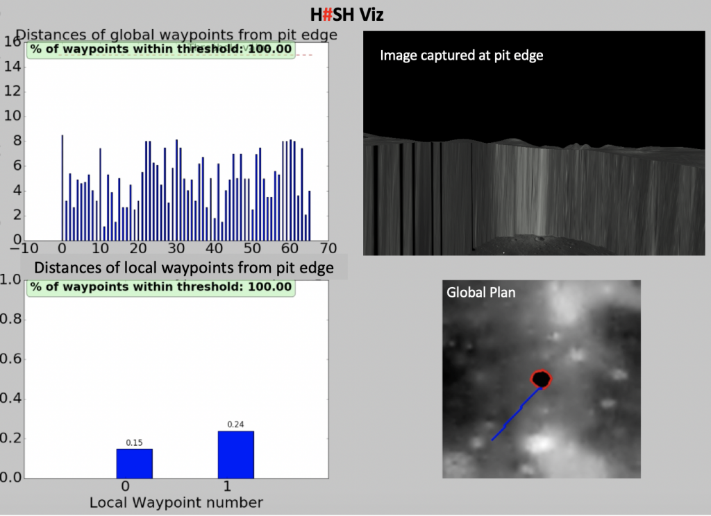
We built a real-time visualization to verify the range and bearing measurements as well as drift between odometry poses, colocalized poses and ground truth poses. Figure below shows our visualization.

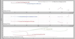
The first graph plots the ground truth range vs estimated range while calculating the running mean error between them. Second graph plots the ground truth bearing vs estimated bearing while calculating the running mean error between them. The third graph shows the trajectory taken by the rover from odometry reading, RTK GPS reading as well as colocalized readings.

Planning in Simulation [12/12/2019]

Simulation Software
For performing planning in simulation, we required the simulator to include a skid steer robot, lunar environment, modelling obstacle distribution and show illumination pattern as per real lunar conditions. We used Webots, in which we used a 2.5D map to model our lunar environment. We generated a pit by approximating it as a polygon circumscribed by a circle of a certain radius. Starting from a point, we go clockwise to perturb the radius of the edge by a gaussian noise. This pit is then moved over to the lunar map and is depressed to a depth. For the robot, we used the existing skid steer robot included in Webots, the Pioneer 3-AT.
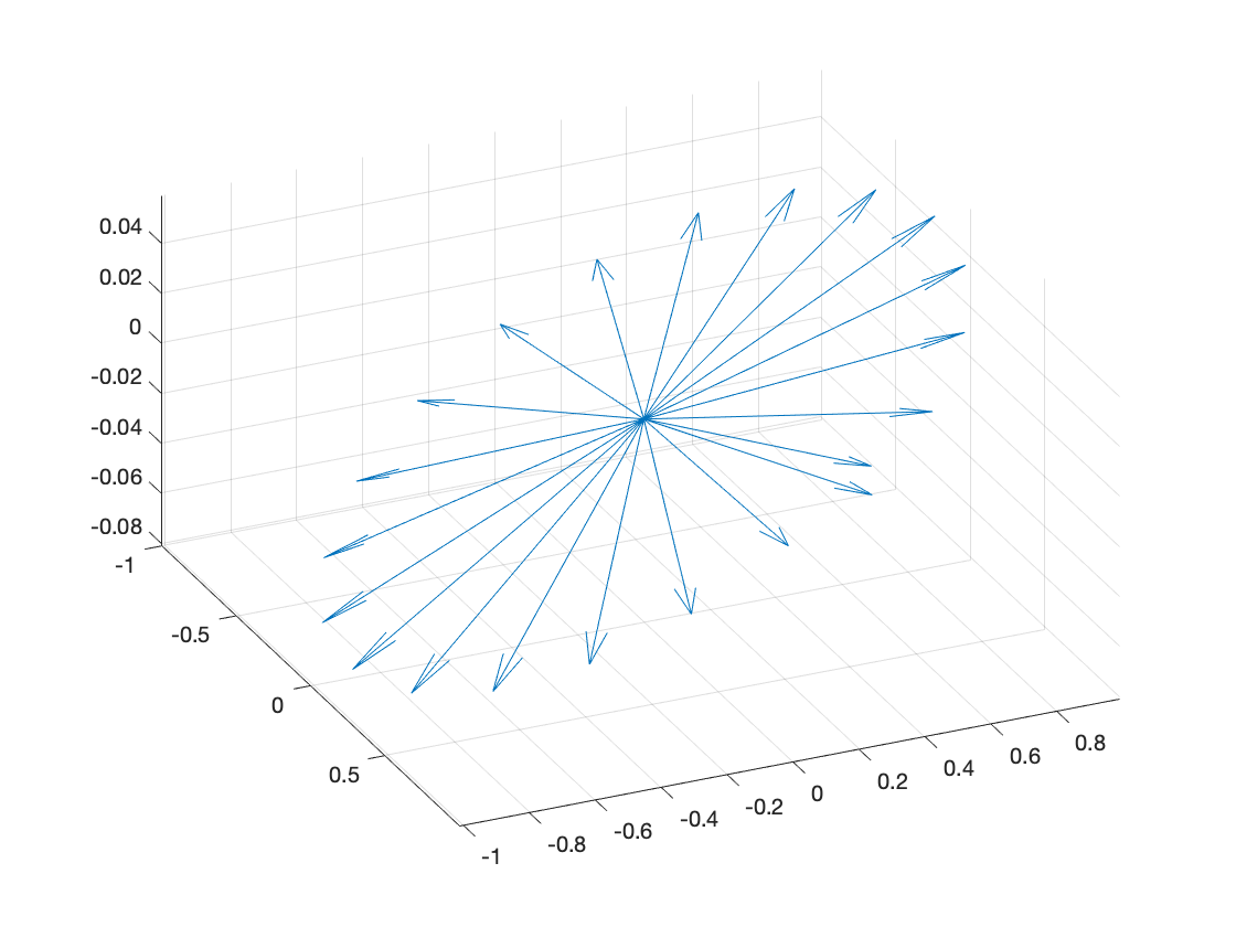
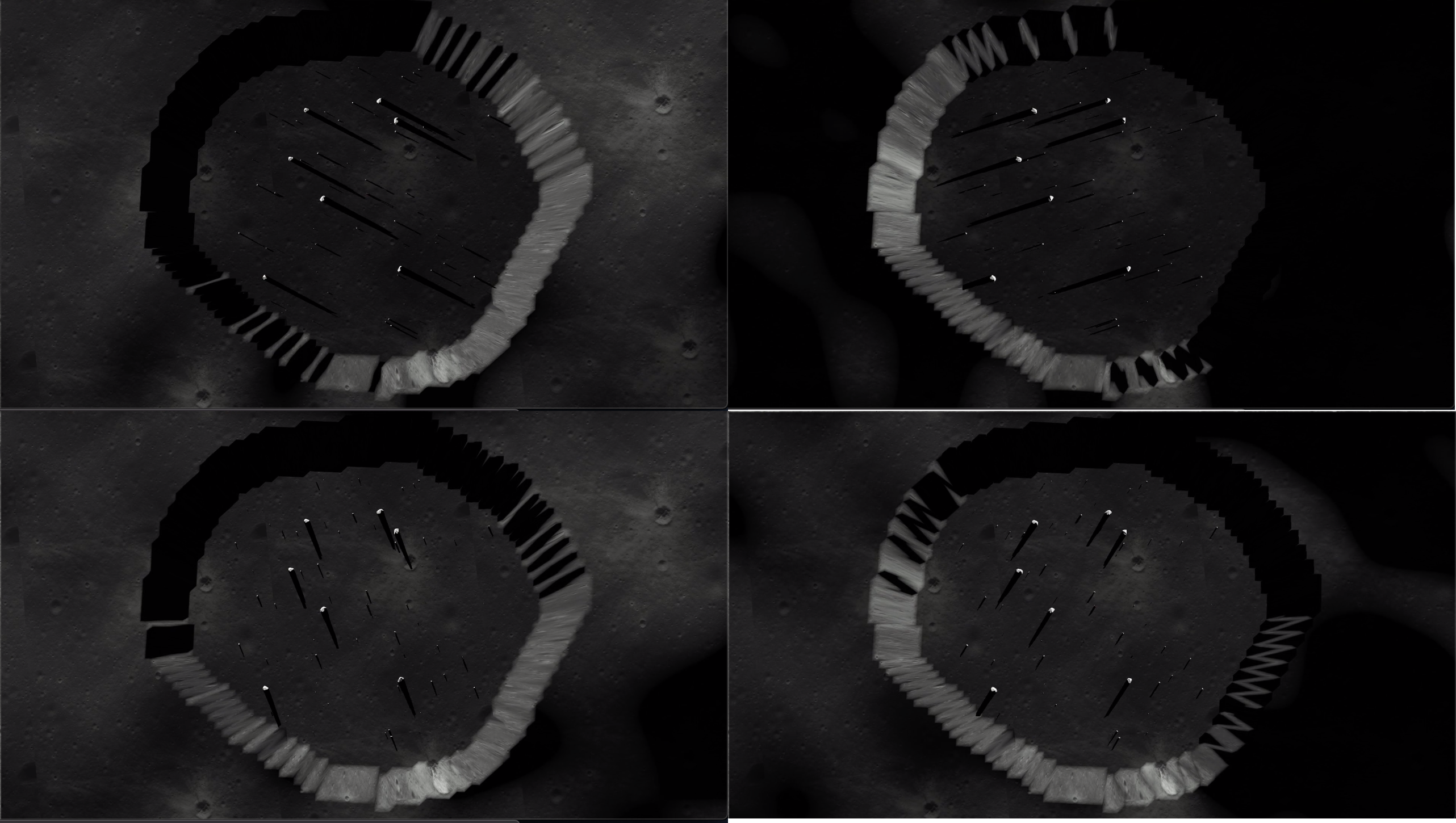
The illumination at the pit at each timestep was calculated based on the relative position between the Sun and the Moon. The NASA CSPICE (Acton et al., 1996) tool provides the vector position of the Sun with respect to the Sun. It also provides the pose of the Moon, with which we calculate the direction of the Sun with respect to a point on the surface of the moon. This vector is then converted to an ENU (East-North-Up) frame of reference. The resulting illumination vectors can be visualized in Figure 10 and the corresponding illumination in our Simulator with the pit are visualized below

Navigation and Controls [12/12/2019]
Navigation subsystem consists of generating the required motor velocity for each of the four wheels in our differential drive robot. We accomplish this task using command velocity generated from the TEB planner. Given a goal waypoint and optimization parameters, TEB planner generates command velocity necessary to achieve the waypoint. The command velocity gives the linear and angular velocity which is further converted to motor velocity using the following formula: –

This left and right wheel velocity are further provided to the robot in the simulator. Webots simulator has an inbuilt velocity control mode for the motors which doesn’t prevent our robot from having jerky motion.
Navigation subsystem also consists of calculating the odometry of our robot. For this, a position sensor (encoders) is installed on each of the wheels. The encoder readings are further used to calculate the odometry of the robot which will be used by the TEB planner as the current location of the robot. Odometry or the current location of the robot was calculated using the following formula

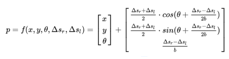
Where x, y, θ is the current pose of the robot and \Delta s_r,\Delta s_lis the right and left encoder readings.

Modelling of noise in odometry
The odometry values received from the encoder values would be ground truth values as those are coming from a simulator. To simulate the noise accumulated in odometry to make our simulator, we model the noise in odometry. To add noise, we model the motion of the robot between two odometry readings as shown in figure below.

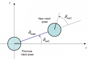
The motion of the robot can be modelled as first rotation \delta_{rot1}, second rotation \delta_{rot2\ }and relative translation \delta_{trans} where

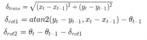
We add zero mean gaussian noise with standard deviation \sigma_{rot1}^2, \sigma_{rot2}^2 and \sigma_{trans}^2 to the above rotation and translation. With updated {\delta\prime}_{rot1},\ {\delta\prime}_{rot2\ },\ {\delta\prime}_{trans} , robot pose with noise can be calculated as follows

The updated odometry values are published over a ROS topic ready to be consumed by TEB planner.

Planning

The Planning stack comprises of three planners 1] Global Planner 2] Local Planner 3] To the pit Planner. Inputs to the planning system are the topographical map of the Moon, a binary map generated based on the elevation gradient and the pit we are targeting. The output of the system will be a global plan and a local plan to reach the destination/next-waypoint taking into consideration all the constraints.

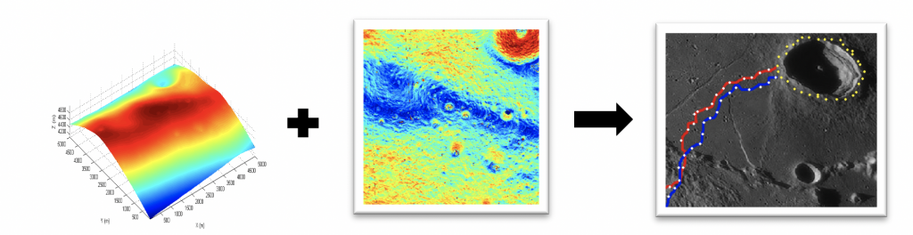
Global Planning

The Global planner differs drastically in the two scenarios mentioned above. While planning the path to the pit, the Global planner takes the topographical map of the moon and plans the shortest path from the lander to the pit while avoiding slopes of gradient 20 degrees. The planner first uses the topographical map to identify the pit based on the elevation gradient. Once the pit edges are identified, waypoints are created around the pit edges, one pixel away from the pit edge. This is done to generate a safe plan later and avoid under any circumstance the catastrophic event of rover falling into the pit. Waypoints that are of extreme elevations are pruned off as they are untraversable. Based on what pit is being targeted a start location is selected for the lander and the same is the start location of the rover as well. The first waypoint around the pit, which the rover should go to from the lander is also determined. For planning a path to the pit, a weighted A* with Euclidian heuristic was used. An implicit graph was used to avoid the overhead of storing the entire map since the entire map was not needed anyways. For around the pit global planning, a weighted multi-goal A* with Euclidian heuristic was used. A weighted cost function that incorporated time to reach vantage point, cost to reach vantage point and extent of coverage in a single lunar day was crafted. The global planner took into account the changing illumination of the Sun and also the velocity of the rover. A factor of pessimism was incorporated to account for the lost time in case the rover has to encounter a local obstacle. The inclusion of this pessimism factor allowed us to run the entire global planner offline. This is of immense importance to planetary and lunar missions as we onboard computation is extremely valuable for these small planetary rovers. So, the global planner does not hog the on-board memory of the rover.

Local Planning
Local Planner: The local planner remains the same in both scenarios. The local planner is primarily responsible for fusing global planner with the local environment and avoid obstacles of height more than 10 cm. The local planner does this based on the cost map generated by perception subsystem.

The system uses a Time-Elastic Band (TEB) planner for local planning. Navigation between the global waypoints contains a lot of intricacies that are taken care of by this planner. The TEB planner takes in the information of the robot-like the type of drive, maximum acceleration, maximum velocity, size of the footprint of the robot. It also takes in a global and a local occupancy map which allows the planner to generate feasible paths. The global map is loaded once but the local occupancy map is updated frequently.
The TEB planner fragments the path into smaller sections and estimated the time to reach the goal based on the rover’s maximum velocity and acceleration. As soon as an obstacle is detected on a previously computed path, a new motion plan is generated to reach the goal in time.
The entire mission can be divided into three stages and transition between these stages is coordinated by a state machine. The first is traversal from the lander to a pit. The rover receives a set of ordered waypoints from the global planner which it tries to accomplish. The last waypoint of this global plan coincides with the first global vantage point around the pit. Once it is reached, the system transitions into the next state, which involves moving closer to the edge of the pit and capturing an image of the illuminated portion of the pit. If this step is successful, the system transitions into the third stage- which involves traversal around the pit from one vantage point to another. Once this is realized the system again cycles to the second stage and this process gets repeated until the entire pit is covered. A system status flag evaluates the success and failure of these transitions. The system shifts to achieve the next waypoint in case it fails to complete either of these transitions. The generated plan incorporates a dense collection of vantage points which have the overlapping field of views. So missing a few vantage points would not impair pit coverage.

To the Pit Planner: It is important to note that the pit edge generated from the LRO global map data is of low resolution. A low-resolution map lacks information that is required to facilitate rover navigation to the edge of the pit. Navigation to the edge of the pit, from the given global waypoints, for capturing images of the inside of the pit, is handled by the local planner. The local planner uses bug algorithm to generate waypoints while keeping the centre of the pit as its goal point. The plan is recomputed after taking a minimum step towards the goal. Once the rover reaches the pit edge (as in figure 9), the plan is aborted.