Camera Perception: Object Detection
We have integrated YOLO-v3 object detector / classifier and SORT tracker (implemented on PyTorch) into a ROS tracker node. The tracker node subscribes to the RGB image from the RealSense camera and publishes object tracking information (object bounding box, class prediction, and incremental object ID — the same ID number refers to the same object that’s being tracked).
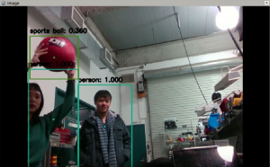
YOLO-v3 is a deep neural network for object detection and classification. In order to detect and classify objects that the drone would likely be encountering / seeing during flight, we created our custom data set and are training a custom classifier on YOLO-v3. The custom training process is based on Darknet features, and the custom detector and classifier is to be trained (to maximize objectness and classification scores on custom dataset). Current object classification classes include balls, people, and drones, though we plan to add new object classes to our custom dataset in the future.
The YOLO-v3 framework is able to reach 30 FPS on our Xavier onboard computer system, which is sufficient for real-time inference.
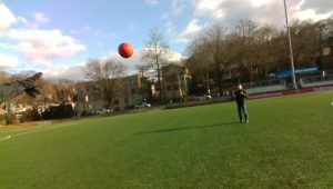
YOLO-v3 inference on custom dataset:
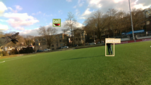
YOLO-v3 running on real-time webcam stream:
Camera Perception: Object Tracking with SORT
With object detections provided in each frame, we can take advantages of this information to “keep track” of our objects. The approach we are using is SORT, which is a Kalman filter based method. Our Kalman filter model includes four states to be predicted, which are x, y, w, h (x, y pixel locations, width and height, respectively). Our model assumes x and y to be constant acceleration, while w and h are constant velocity. That yields 10 state variables (x, y, w, h, dx, dy, dw, dh, ddx, ddy) to be kept track of. The model definition is shown in the diagram below.
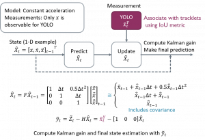
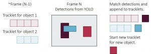
In each frame (time step), we make a prediction of the current “tracklets”, which are the object trajectories present in the camera frame, in the prediction phase of Kalman filtering. For the update phase, we take advantage of the new detections received from the YOLO network and use them as the “measurement” of our four states (x, y, w, h). Based on the Kalman gain and variables, as well as the class predictions, we can associate tracklets and detections and update the former with the latter.
To associate detections to tracklets, there are two metrics we are using, the first is the class prediction — only consider associating tracklets and detections with the same class label. The second metric is the IoU (intersection over union) — if the predicted and measurement bounding boxes have an IoU score above certain threshold, we then establish the association. The tracking pipeline is shown in the diagram below.
A short summary for the SORT tracking pipeline:
- At each timestep, make predictions of each tracklet / object.
- Receive detections from YOLO-v3.
- Compare new detections to existing tracklets
- Match existing tracklet: assign detection to tracklet & update tracklet with detection.
- No match for detection: Consider this as a new object and create new tracklet to keep track of it.
- No match for tracklet: Set tracklet to inactive.
- Cleanup: If tracklet is inactive for a certain timesteps, consider object has left the field of view and remove tracklet.
We have now integrated the YOLO detection and SORT tracking pipeline into a ROS package.
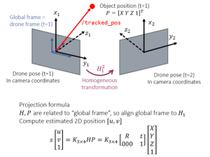
Object tracking: SORT with drone motion
The second version of the SORT tracking algorithm uses the drone’s pose to eliminate noise. Testing found rapid changes in the drone’s position caused the standard SORT tracker to lose tracklets. After publishing the 2D tracklets, each object gets its 3D position estimate (introduced in section below). The new tracker node subscribes to the 3D object positions and drone motion topics, and then uses camera projection to estimate the “motion” of the bounding box in 2D between the current and previous timesteps. This estimated motion is then taken into account as the “control input” term of the Kalman filter.
The computation pipeline of the control input term is illustrated in the diagram below.
Lidar & Sensor Fusion
We have created ROS package which handles all of the lidar point cloud processing as well as sensor fusion.
This packages subscribes from two sources, the bounding boxes output from the YOLOV3-SORT package and the raw point cloud data published by the Velodyne.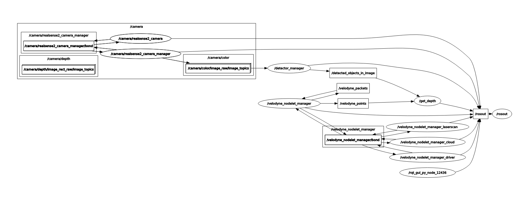
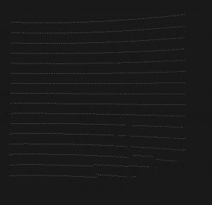
After receiving the raw lidar point cloud, the ROS node first filters the point cloud to a 70 degree field of view to match that of the Realsense camera’s. In addition, any points outside the 10 meter radius are filtered.
-
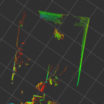
- Original Point Cloud
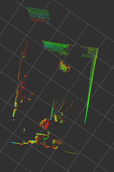
-
- Cropped Point Cloud
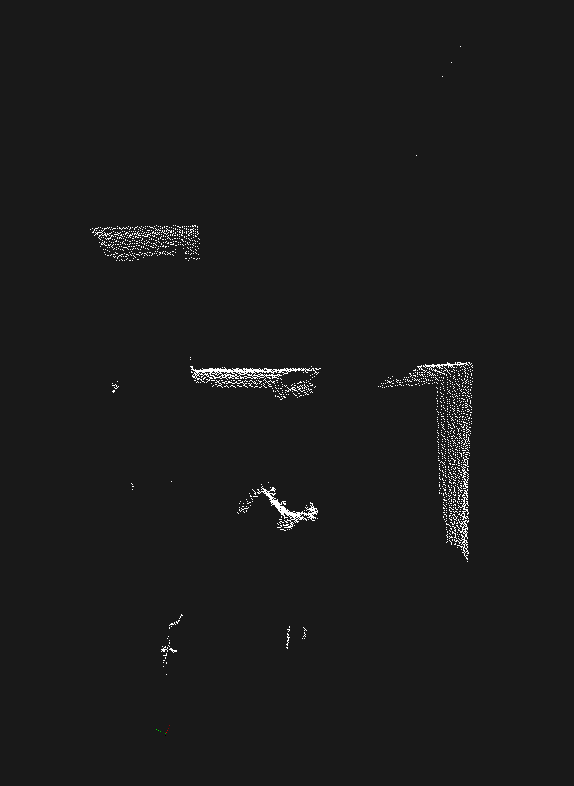
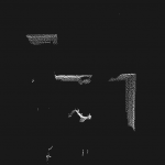
We apply an Extrinsic transformation matrix to the point cloud to place it in the same coordinate as the Realsense camera. We then apply the intrinsic matrix of the camera to the point cloud points to project the 3D points onto a 2D image plane.
Projected Point Cloud
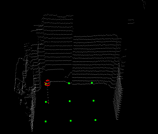
We add a patch of 10 pixels around the bounding box output by the detector/tracker, and then segment out all the corresponding point cloud points inside the enlarged bounding box. These points are highlighted in red on the left side in the figure below.
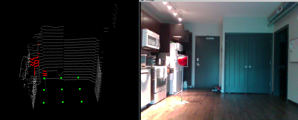
An additional cluster filtering is applied to all the points inside the bounding box to separate the points corresponding to the object of interest and background. We calculate the centroid locations of the clusters by taking an average of all the points within the clusters and pick the one that is the closest to the lidar. The result of the cluster filtering is shown below. The point clouds corresponding to the background are no longer highlighted. A additional step of Ransac base ground plane detection and filtering was applied to remove all the points on the ground plane.
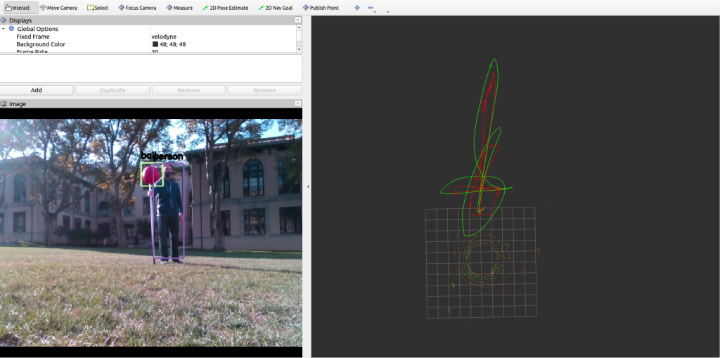
Lastly, we take the average of the coordinates of all the points corresponding to the object of interest to obtain the estimation of the object location in the local frame. The local frame position is then transformed into the global coordinate frame by applying the position and rotation transformations published by the DJI SDK.
The final result could be seen in the figure below. The red marker marks the position of the drone and the green markers mark the position of the detected person and the ball. You can see that the detected objects are placed in the correct position with respect to the drone in the world frame.
Lidar Perception: Trajectory Prediction
The trajectory prediction package subscribes to the topic published by the lidar process node. The data is in terms of the scan by scan positions of the detected objects. Each of the detected objects is assigned a unique object id. Within the trajectory prediction node, an object position dictionary is maintained. The keys of the dictionary are the object ids and the values are arrays of the object position along with corresponding timestamps in the past. The outdated position information in each of the arrays in the dictionary are constantly being cleared so that only the most recent positions are used to make the prediction. A custom implemented polynomial regression function would then fit an Nth order polynomial between the past positions and the corresponding time steps. An array of interpolated future time steps passes into the polynomial model to obtain the future trajectory. In Fig. 11, the red trajectory corresponds to the detected position from the lidar process node. The green trajectory corresponds to the polynomial trajectory from the trajectory prediction node.