Design Brainstorming

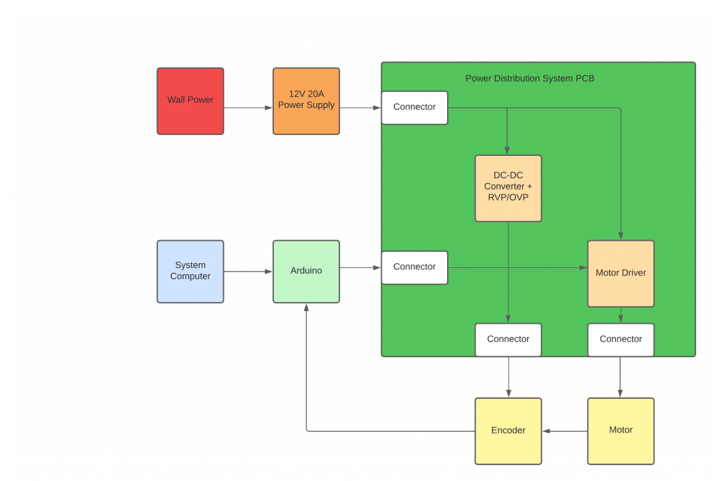
PCB Design

High-level Diagram Showing General Layout of PCB for Powering and Controlling Motor

End-Effector Design

Perception Subsystem

Brainstorming for Perception Software Subsystem

Planning Subsystem

Controls Subsystem

Miscellaneous

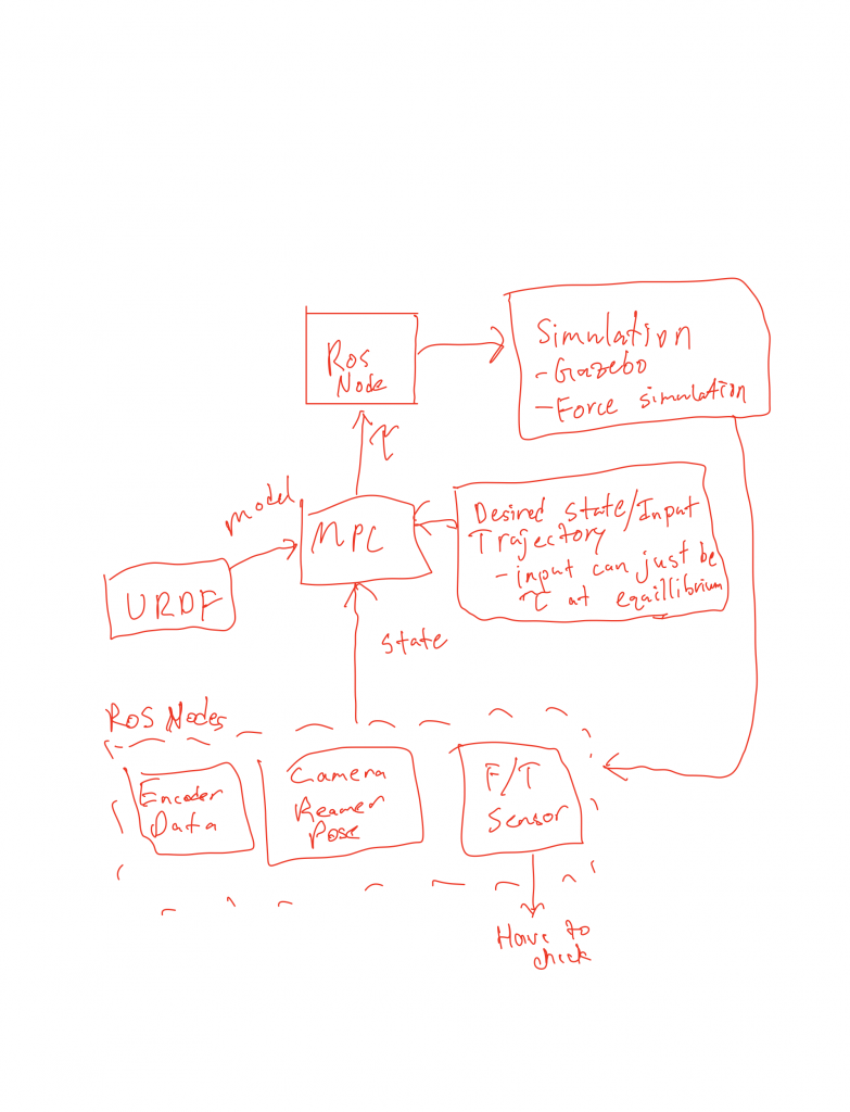
MPC Brainstorming

Deciding the Controller and Formulating the Optimal Control Problem

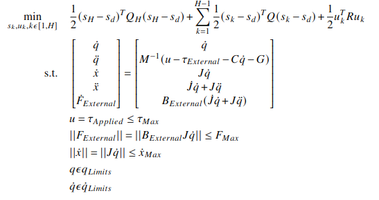
After surveying the possible controls algorithms that could be used for this system, a Model Predictive Controller (MPC) was decided as the best controller because of our system constraints and goals, changing system dynamics, and that MPC can take multiple inputs. Using classic manipulator dynamics, the system dynamics were determined. Constraints were determined based on literature research and system requirements. For the objective function, a tracking objective was chosen, minimizing the error along a desired trajectory while meeting constraints. Figure 16 shows the Optimal Control Problem.

Implementing the Dynamics Modeling of the Kinova Gen3 Arm

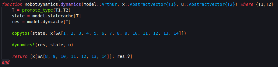
The dynamics function of the Kinova Gen3 Arm was implemented using the Julia Language and the RigidBodyDynamics.jl library. This library parses the URDF of our model and builds a joint-linkage tree, storing the mass and inertias. Given the joint positions, joint velocities, external wrenches, and input torques, the library has dynamics functions that can calculate the joint accelerations. Figure 17 shows the currently implemented dynamics function.

Figure 17. Implementation of System Dynamics Using RigidBodyDynamics.jl

Implementing the MPC

Using the RobotDynamics.jl, TrajectoryOptimization.jl, and Altro.jl, the MPC was implemented, organizing a trajectory of desired states and desired inputs over time, setting up the Tracking Objective function, and setting up the System Constraints defined above in Figure 16. The most challenging part of setting the MPC up was providing a good initial guess for input torques for the solver to converge. The best initial guess was providing gravity compensation torques for the initial position of the manipulator in the trajectory. Figure 18 shows the implementation of the objective function and joint position and velocity constraints. Figure 19 shows an offline simulation of the MPC output, which had a very low tracking error (less than 0.001 mm and less than 0.5 degrees error of end-effector pose).

Figure 18. Implementation of Objective Function and Constraints

Figure 19. Offline Simulation of MPC Output Following a Trajectory

Integrating the MPC into ROS

RobotOS.jl was used to integrate the MPC into ROS within the Julia Language, and is a wrapper for PyROS, allowing for the node to subscribe and publish messages within ROS. Two nodes were written as part of the controller: an MPC node to solve the optimal control problem given the current state, desired trajectory and system constraints, and a Controller node which sends the appropriate torques to the effort controllers in simulation or hardware.

Integrating the Motion Planner and Simulating in Gazebo

After writing the ROS nodes, the MPC was integrated with the Motion Planner subsystem and with the Gazebo simulation and joint effort controllers at a rate of 20 Hz (will increase later). This enabled real-time simulation and testing of the MPC, which revealed challenges with getting the MPC to converge on time.

Implementing the PD Impedance Tracking Controller

Since there were issues with getting the MPC to converge, a PD Impedance Tracking Controller was developed in parallel. Using the RobotDynamics.jl, the error in desired joint positions and velocities were given to the controller to determine the desired joint accelerations. Using the desired accelerations, the desired torques were calculated using inverse dynamics within the library, which uses the Recursive Newton Euler Algorithm. These torques are then provided to the effort controllers. Figure 20 shows the real-time simulation of the PD Impedance Tracking Controller following a straight-line trajectory in Gazebo.