System Implementation

Fall 2022

Perception and Sensing Subsystem

Interfacing with the Camera

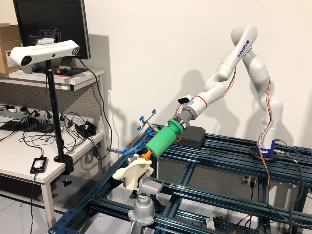
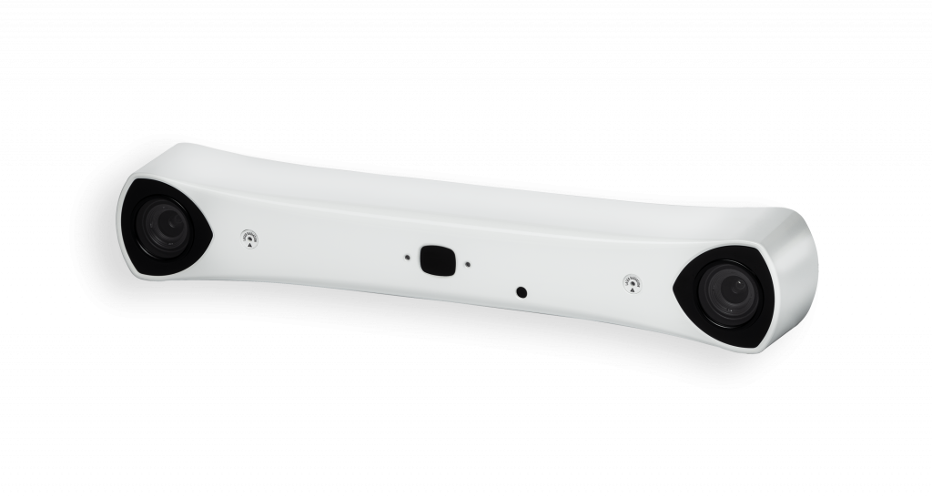
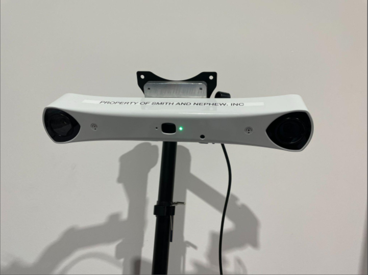
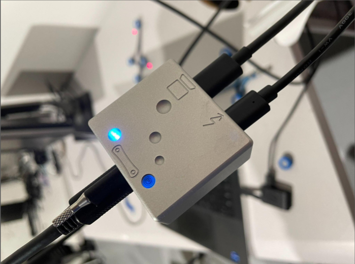
The development of the perception and sensing subsystem began with interfacing the Atracsys Sprytrack 300 camera shown in Figure 1. The camera was set up in the lab workspace using the provided power injector and cables. A stand was procured and a camera mount was designed and manufactured to hold the camera. It was mounted to overlook the workspace. The setup is shown in Figure 2.

Figure 2B. Power Injector for Atracsys Camera

Marker Geometries and Tracking

The camera is able to track a unique geometry of reflective/fiducial markers. This helps the system determine and track the 6DOF pose of various components in the workspace- registration probe, pelvis, and the robot arm end-effector. The information about the unique fiducial marker geometry is stored in a .ini file that is loaded into the camera software.

Understanding the Camera Software

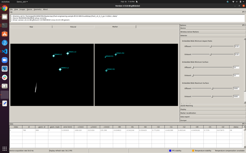
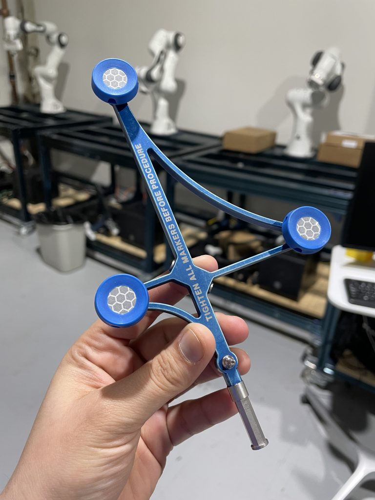
Initial experiments with the camera involved understanding the provided Atracsys SDK, a C++ library that interfaces with the camera and allows for data collection, detection, and tracking. The code sample and Atracsys SDK GUI were very helpful in experimenting with the camera to understand its various capabilities. Figure 3 shows the Atracsys SDK and the reflective markers used. Figure 4 shows the marker poses being detected in the SDK GUI.

Figure 3B. Marker Array Used in Picture Shown on Left

Interfacing the Camera Software

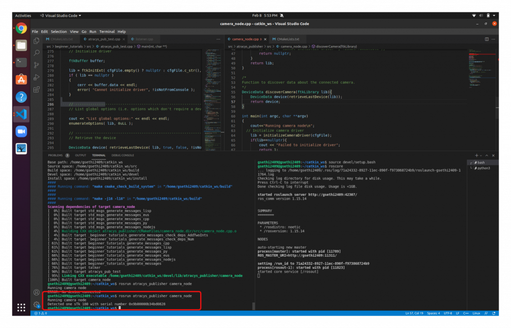
The underlying framework of the entire system is based on ROS. Therefore, the Atracsys SDK libraries were interfaced with ROS using C++ and CMake. This was pretty challenging given the complexities of linking with static/dynamic libraries and debugging cryptic CMake errors. However, after persistent efforts, we successfully linked the Atracsys libraries with ROS. As a test, we wrote a simple ROS node that would discover the camera and load a marker geometry. The test was successful and is shown in Figure 5.

Figure 5. Simple ROS Node to Test Atracsys + ROS Linking

Tracking Markers and Publishing Realtime Poses

The geometry files were loaded into the ROS node and the Aytracsys APIs were used to track the marker geometries. The 6DOF poses were converted to standard ROS message types and published in real-time while maintaining the camera’s FPS of ~50. The frames were visualized in RViz. This is shown in Figure 6.

Figure 6. Frames of Markers Visualized in RViz

Sensing and Tracking

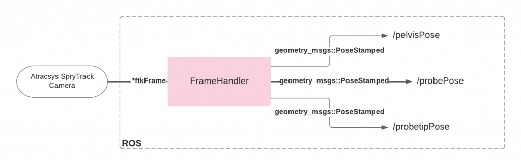
Primarily, the Atracsys Sprytrack 300 camera tracks predefined geometries of reflective fiducial markers. The geometries are loaded into the FrameHandler which is responsible for communicating with the linked camera libraries from within ROS, receiving tracking measurements and continuously making them available on ROS topics for the other subsystems. The 6-DoF poses of the objects are published as standard ROS message types at 55 FPS. The pelvis is continuously tracked by a PelvisTracker. If the change in pelvis pose is greater than the position and orientation error tolerances, the perception subsystem indicates, through a Boolean ROS message, that the pelvis pose error has been detected. In this case, the dynamic compensation is expected to be triggered. The workflow of the FrameHandler and PelvisTracker are shown in the figures below.

Sparse Pointcloud Collection

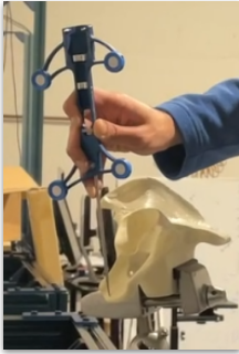
As an initial calibration step, the surgeon will perform landmark collection. This means that the surgeon will use a registration probe (Figure 8) in order to pick points of the pelvis that will be used for registering the real human pelvis with the pre-operative pelvis 3D scan. Technically, this would mean that the perception pipeline must allow for the surgeon to collect a pointcloud.

As an initial guess for the registration pipeline, the surgeon will be able to pick 5-10 by hitting “Enter” on the keyboard.

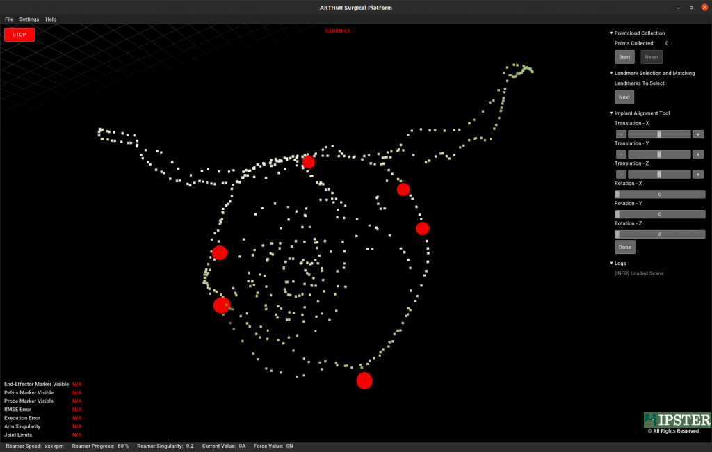
Figure 8A. Registration Probe Visualized in RViz

Continuous Dense Pointcloud Collection

The surgeon will then pick a more dense pointcloud of over 1000 points. This would mean sliding the registration probe on the pelvis to collect points. Both pointcloud collection functionalities have been successfully implemented and tested. This can be seen in Figure 9.

Understanding Open3D I/O

The registration pipeline in perception and sensing began with the understanding of how to read meshes and pointclouds into Open3D. Here, we realized that meshes need to be saved as ASCII files rather than binaries for it to be read into Open3D. Once this was done, conversion from pointcloud to meshes and vice-versa was explored. Operations on pointclouds such as changing colors, scale, transformation density and visualization using the Open3D viewer were explored.

Figure 10. An off-the-shelf model of the pelvis loaded into Open3D

Problem Domain Familiarization

A basic understanding of the registration problem was acquired by reading relevant literature. Various options to perform registration were explored, and the most suitable option for our problem was chosen to be Iterative Closest Point (ICP). The ICP based registration tutorials on the Open3D website were implemented with the help of example pointclouds provided. The various hyperparameters used in the registration process were explored to get an understanding of the important features to be tweaked.

Acquiring Mesh of Pelvis

The pelvis model was 3D scanned using a Konica Minolta 3D scanner from a lab at CMU. This was then post-processed to fill in holes and eliminate other undesirable artifacts. This was then converted into an appropriate ASCII mesh file that could be loaded into Open3D.

Preliminary Registration Test

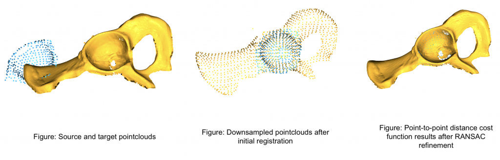
The scanned mesh was loaded into Open3D. A part of the pointcloud was extracted out to represent the sample we would acquire from the registration probe. This sample was translated and rotated using an arbitrary configuration. Some modifications were made to the reference code in the Open3D tutorials and hyperparameters were tweaked to make the implementation work for our problem.

Figure 11. Registration on simulated pelvis model (source not obtained from probe)

Initial Guess for Registration

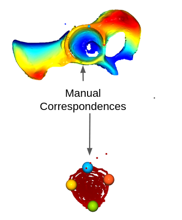
ICP requires an initial guess of the transformation between the source and target pointclouds for registration. We obtained this guess using manual correspondence matching. A minimum of three points were required to solve for the translation and rotation between the source and target pointclouds. Once this was acquired, it was converted to a homogeneous transformation matrix and fed as input into the registration algorithm. The figure below shows the correspondence matching step between the source and target pointclouds.

Registration of Real Pointclouds

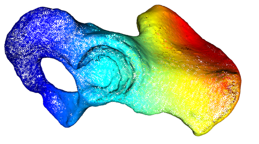
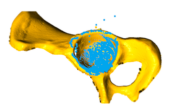
Using the previously described method of collecting dense pointclouds, we were able to acquire an accurate representation of the acetabulum of the model pelvis. This, when coupled with the initial guess from manual correspondence matching, and some hyperparameter tuning gave the transformation between the simulated pelvis model and the real pelvis. This transformation will be used to determine the end-point for reaming as the input into the planning module.

Figure 13B. After Registration (Source Acquired from the Registration Probe)

Controls Subsystem

Connecting Kinova Gen3 with the Desktop

The kortex driver written by Kinova automatically loads when an arm is connected to a computer. For the computer to detect the arm, the IP address and the subnet mask has to be configured. Once configured, the kortex driver loads successfully and commands can be sent to the arm via ethernet. We can also access all the information on current joint states, camera view etc. using the Kinova Web API.

Controller

The controls subsystem is responsible for three major functions: Free Motion Mode which allows the surgeon to move the reamer end-effector close to the site of reaming before starting the surgery, Autonomous Control Mode which executes the trajectory given by the planning subsystem, and Dynamic Compensation which adjusts and aligns the end-effector’s pose with the pelvis’s pose if the pelvis moves during the reaming operation.

Free Motion Mode

For the Kinova Gen 3 arm (7 DOF), Free Motion Mode is already implemented into the base firmware of the arm as a joint admittance mode, which can be activated by pressing a button on the last link of the arm or activated through their API calls. This made integration into our system fast and easy.

Autonomous Control Mode

Arm Controls

For Autonomous Control Mode, the controls subsystem is using Kinova’s Joint Velocity Controller API as the low-level controller to track the acetabulum and align the end-effector markers to the camera. For our system, we are using two isolated controllers: one for the arm to align the end-effector to the acetabulum and align the end-effector markers to the camera, and one for performing the force-controlled reaming operation.

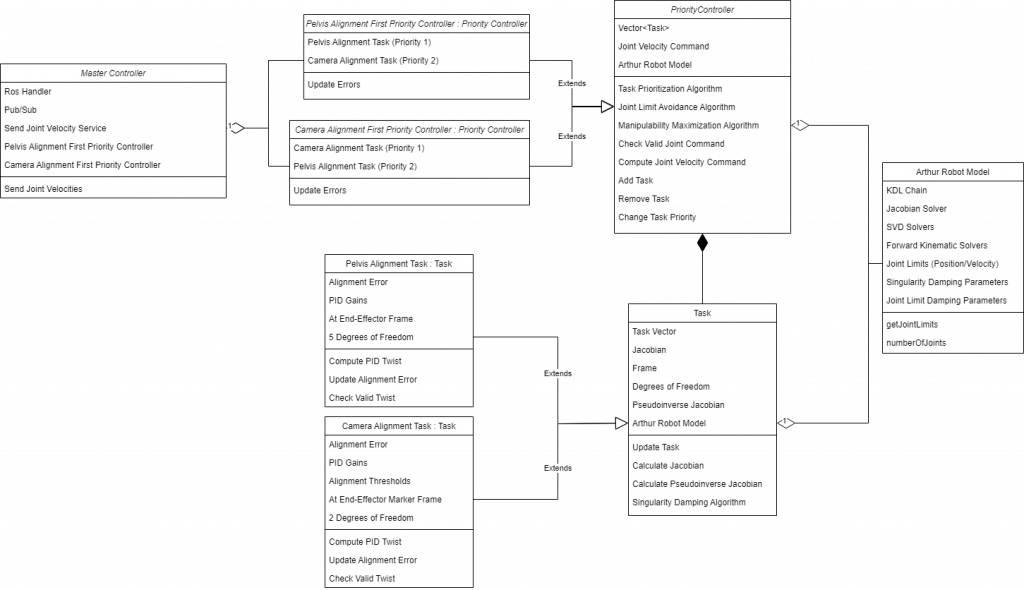
For the first controller, we are using a Task Prioritization Framework, allowing us to take advantage of the redundancy of our arm and perform multiple tasks simultaneously. We have two main tasks to execute; the first is to align the end-effector to the acetabulum, and the second is to align the end-effector markers to the camera. Since the end-effector is doing the reaming operation, force-based control is not as much of a concern for this specific controller since it will be handled in the end-effector controller, allowing us to use joint velocity control for a faster response than the previously used Wrench controller. For both tasks, a PID controller is utilized to create the desired twist at each respective task frame based on the error of frame alignments with their desired frame. Because the reaming end-point is only generated once relative to the pelvis markers, no re-planning is required so we can perform real-time dynamic compensation for any patient movement. A basic implemented UML diagram for the task prioritization framework is shown below.

Figure 16. UML Diagram of Task Prioritization Framework

The acetabular alignment task has been implemented as well and can be seen below. The position (blue) and orientation (red) steady-state error goes to zero if the pelvis remains stationary.

Figure 28. Acetabular Alignment Task: Arm is aligning with a frame relative to the pelvis.

Figure 29. The Steady State Error of the Task shown in Figure 28. Blue is Position Error, and Red is Orientation Error.

With multiple tasks, we can see how Task Prioritization works. In the figures below, we have a pelvis alignment task as the highest priority task, with a camera alignment task, joint limit avoidance, and singularity avoidance task as the proceeding lower priority tasks.

Figure 34A. Task Prioritization With Pelvis Alignment, Camera Alignment, and Singularity Avoidance

Figure 34B. Camera Moving During Surgery

Figure 34C. Arm Adjusting to Camera Movement in Figure 34B.

Figure 34D. Singularity Avoidance – Maximizing Manipulability by Moving Arm in Redundant Space

In the figures below, we also have implemented singularity damping, to increase controller stability at singularities, joint limit avoidance to avoid joint limits and use other joints when necessary, and collision avoidance to stop self-collisions.

Figure 35. Joint Limit Avoidance. Joint 2 is hitting its limits and the controller is using other joints to follow the pelvis.

Figure 36. Singularity Damping to make the controller more stable at singularities.

Figure 37. Collision Detection with the table to avoid collisions with pre-known environmental objects.

Figure 38. Collision Detection with itself to prevent the controller from having the robot hit itself.

End-Effector Controls

High-Level Overview

The end-effector controls involve using our custom end-effector hardware to achieve the necessary reaming motion to complete the operation. Given a surgical plan (i.e., position and orientation of the implant in the pelvis), the arm controls to ensure that the reaming end-point is at a fixed distance from the reaming tool. Once the arm positions itself in this pose, it sends a reaming command to the end-effector through a ROS topic. At this point, the end-effector controls take over the operation while the arm controls continue to maintain the pose relative to the pelvis. In the event that the arm error goes above a 2 mm or 1.5 degree threshold, the end-effector will retract and wait for the arm to realign below the error thresholds.

Current Sensor Integration

The hall-effect current sensor in our end-effector reads the current drawn from the linear-actuator motor. This current measured is proportional to the axial force being applied by the linear actuator on the saw-bone. To begin with, we first calibrated the current sensor by applying a known amount of current and measuring the corresponding value of analog reading between 0 and 1023 from the Arduino Mega. We then determined a linear relationship representing the transfer function relating the applied current to the observed voltage in the sensor.

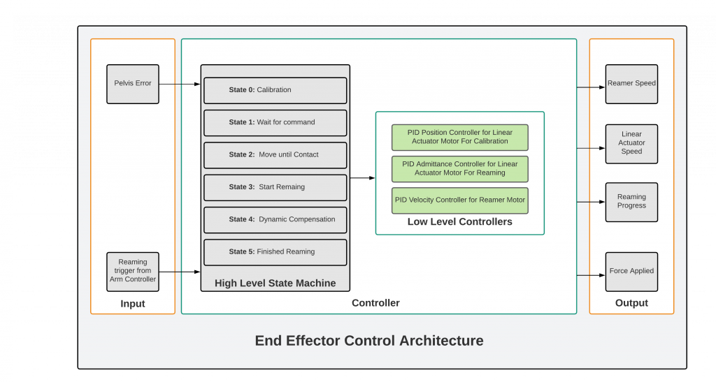
Control Architecture

The general objective of this controller involves being able to actuate the linear actuator until it reaches the reaming endpoint while maintaining a predefined amount of axial force, and allowing the reamer to rotate at a predefined constant velocity. Our controller has a high-level state machine that includes the following states:

State 1 – Calibration: This is a calibration routine wherein the linear actuator moves back until it hits the limit switch. This initializes the position of the end-effector that will be tracked as it actuates during reaming.

State 2 – Wait for command: This is an idle state where the end-effector waits until it receives a command to start reaming from the task prioritization controls.

State 3 – Move until contact: Once a command is received for reaming, the linear actuator moves until it makes contact with a given amount of force against the acetabular surface.

State 4 – Start reaming: Once contact is made, the reamer motor turns on and maintains a constant reaming velocity until the goal state is reached or dynamic compensation becomes necessary.

State 5 – Dynamic Compensation: When the pelvis error exceeds the predefined position or orientation error thresholds, the end-effector retracts to allow repositioning and then subsequently changes state to continue the reaming process as usual.

State 6 – Finished reaming: Final state when the reaming is completed.

These high-level states are used to determine the respective motor position and velocity commands for the linear actuator and reamer motors respectively. These are executed by the PID position and velocity controllers for the linear actuator and reamer motor respectively. The flowchart in the figure below summarizes the functionality of our end-effector controller.

Figure 34A. End-Effector Controls Architecture

The figure below shows the Move Until Contact and Start Reaming states of the state machine. It also shows the force control in effect, moving the reamer back if too much force is applied.

Figure 34B. Move Until Contact and Start Reaming States – Force Control

Watchdog Module

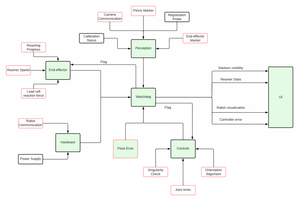
The watchdog node would be the first node to be launched on the system. The watchdog would monitor the health of all subsystems by mainly checking the streams via which each subsystem passes information. The perception subsystem sends information via ROS topics which would be monitored to detect any loss in communication. The status of each of these streams would be seen on the UI as the health of the perception subsystem as a whole. If any of the communication streams are broken, the procedure will not continue. If the health of the perception subsystem is good, then the watchdog will send a boolean flag to the controls subsystem indicating the health, which will allow the controller to start the end-effector alignment task. While the controller is aligning, the watchdog will keep track of the topics exposed by the controller to monitor joint limits, singularities, and the error between the desired and current orientation. If any of these parameters are abnormally wrong, the controller by itself would shut off. In case the controller doesn’t shut off, the watchdog will shut the arm down through a software e-stop (as shown in Figure 33B and 33C). If the parameters from the controller are healthy, the watchdog will send a flag to the hardware subsystem indicating the health of the other subsystems and the progress of the alignment operation. Once the end-effector starts the reaming process, the watchdog will track the reamer speed and the reaming progress. If the reamer is running at a speed higher than the safe threshold, then the watchdog will shut the reaming motor. Similarly, if the reamer remains on long after the reaming operation is completed, the reamer motor will be turned on. The figure below shows a high-level diagram of the Watchdog Module implementation and how it interfaces with other subsystems.

Figure 33B. Watchdog Stops Arm Controller When Pelvis Not Visible

Figure 33C. Watchdog Sets E-Stop When Pelvis Not Visible

Hardware Subsystem

Designing Atracsys Camera Mount

The development of our hardware subsystem started with the creation of an adapter to connect the Atracsys camera to a VESA mount, allowing for the camera to be easily adjusted. The design was created using Solidworks and the part was manufactured in the RI machine shop out of aluminum. The finalized part can be seen in Figure 2A.

Setting Up Vention Workstation

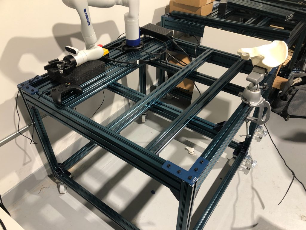
For testing purposes, we needed a consistent workstation that was large enough to accommodate a Kinova Gen-3 arm, and was adjustable to suit any changes to our hardware setup. With some help from Professor Oliver Kroemer, we were able to receive and set up a Vention table to be used as our workstation. Our finalized workstation including a sawbone pelvis can be seen in Figure 22.

Receiving and Setting Up Robot Arm

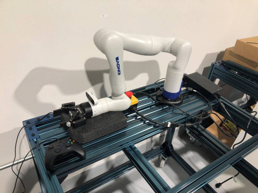
It took a while to receive our Kinova Gen-3 arm. However, once we did it was relatively easy to set up and secure to our Vention workstation. Out of the box, we were able to control it in free motion mode using the cartesian and joint state buttons on the end-effector of the arm, allowing us to adjust the arm ourselves. Furthermore, the arm was also able to be controlled using an included Xbox controller. Figure 23 shows the robot arm connected to our workstation.

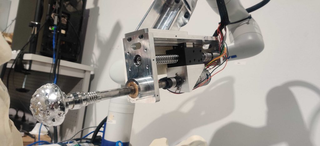
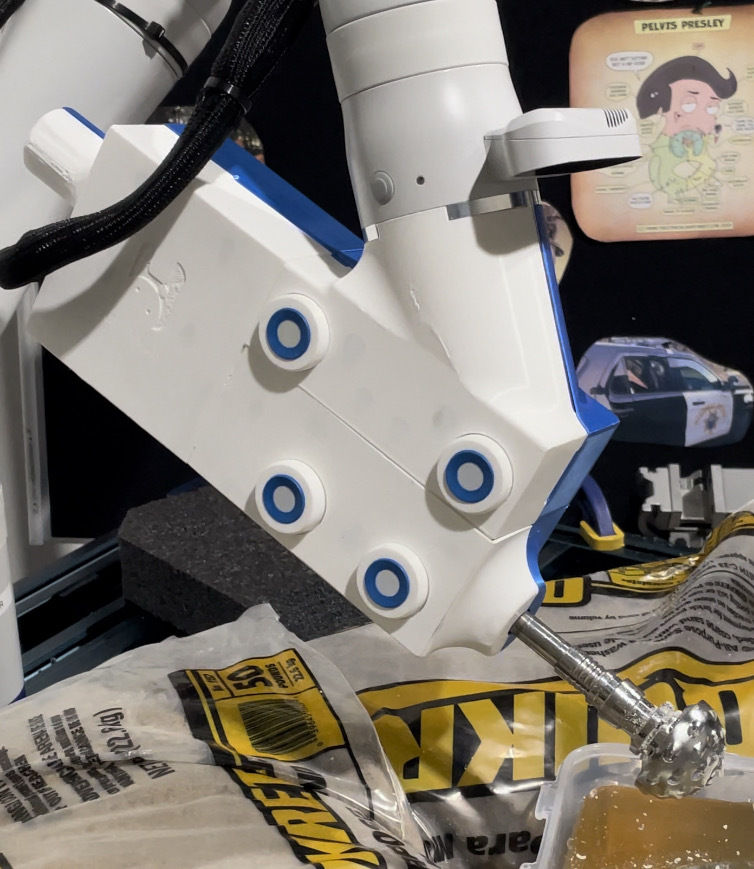
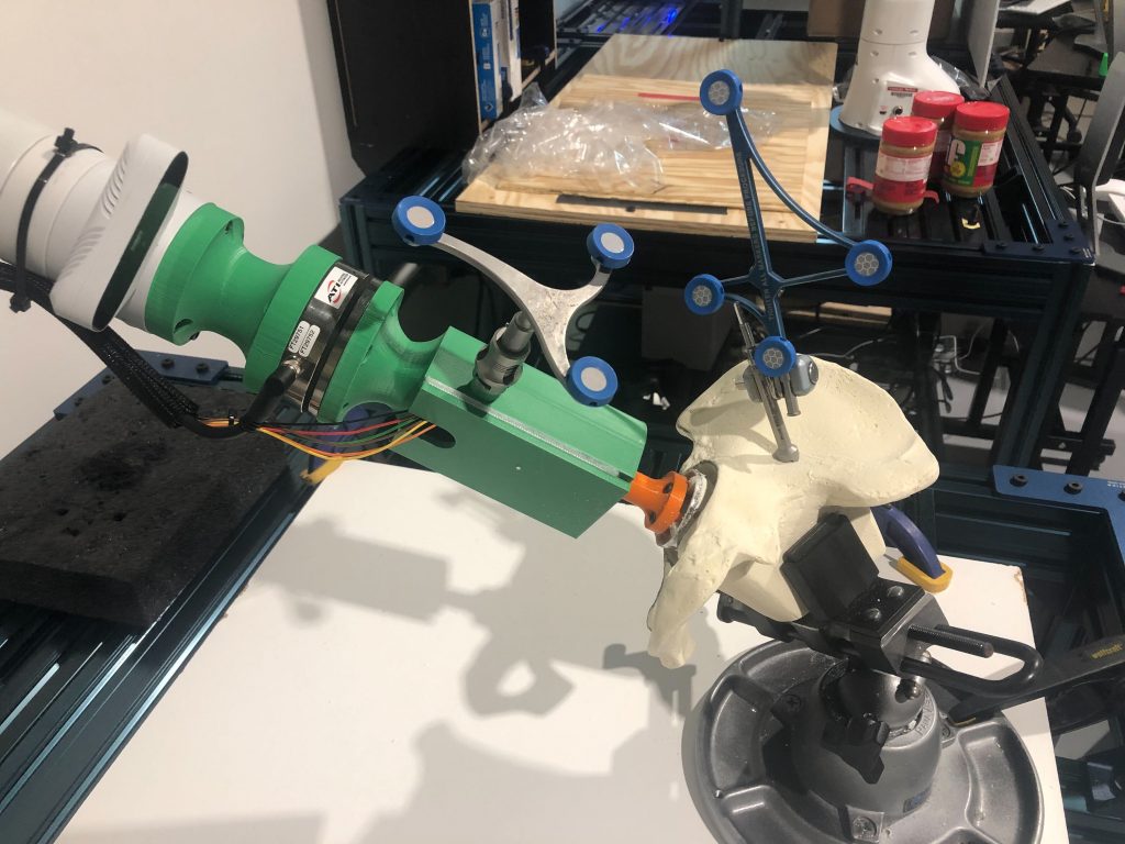
Figure 23. Kinova Gen3 Connected to Workstation

Designing the Reaming End-Effector

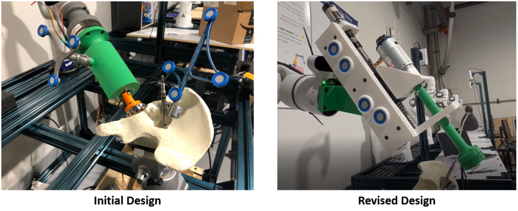
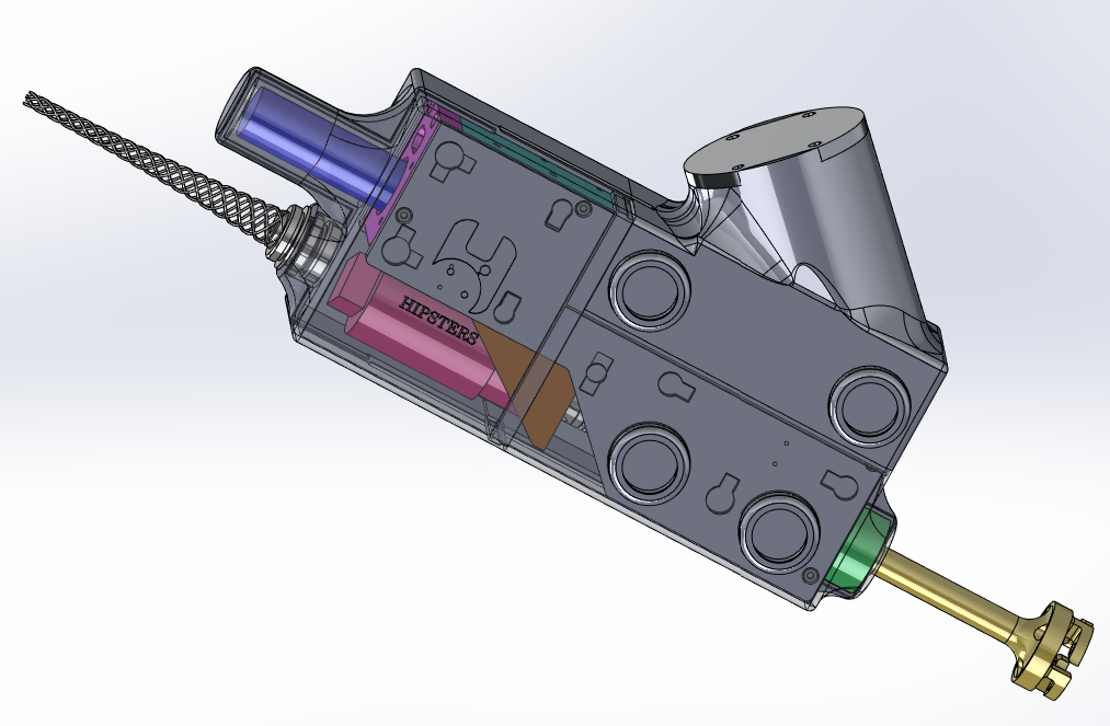
We were dissatisfied with the performance of our initial end-effector, and as such decided to move forward with redesigning our end-effector during the fall semester. Our initial design was relatively simple, just adapting a motor to be axially aligned with the final link of the robot arm which could spin as commanded by an Arduino. The problems with this initial design were that we lost degrees of freedom in our arm by having the end-effector axially aligned with the final link in the robot arm, the end-effector often shook during reaming, and the arm often had to be positioned awkwardly to ream the acetabulum. To solve these problems, we decided to move towards an angled linearly actuated design which allowed us to solve these problems. With an angled design we are no longer losing degrees of freedom and forcing the arm into awkward positions, and with a linearly actuated design, we allow the arm to only position the end-effector and perform dynamic compensation instead of relying on it to also apply force to the acetabulum for reaming. Our design utilizes a linear rail actuated via a ball screw, DC gear motors with encoders, limit switches, and potentially load cells. After we validated that our design was functional with 3D-printed parts we decided to manufacture some of the structural components out of aluminum to further decrease vibrations in our system. Figure 30 shows our previous end-effector design as compared to a 3D-printed prototype of the final design, Figure 31A shows CAD of the current system and Figure 31B shows the finalized manufactured end-effector. Figure 31C shows a cover for the end-effector to enclose the actuation components and create a more professional final product. It uses magnets to make it easily removable, and 3D-printed threads to mount the reflective markers into the end-effector.

Figure 30. End-Effector Designs. Spring 2022 Design on the left, and Fall 2022 Design on the right.

Figure 31A. The current end-effector design.

Figure 31B. Manufactured end-effector design.

FIgure 31C. Manufactured End-Effector with 3D-Printed Cover

Electrical Subsystem

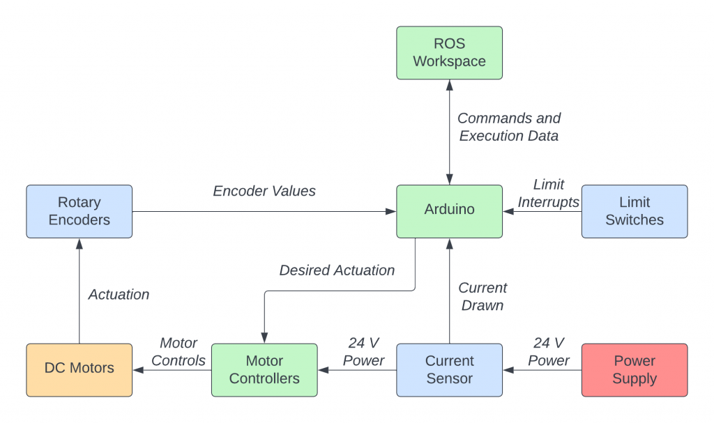
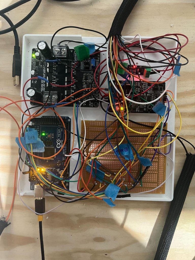
The old electrical subsystem and PCB design are shown in the Spring 2022 section below along with its full integration with the hardware and system. As a result of the update to our end-effector and the overall status of our electrical system from Spring (the PCB we designed for our project largely became unnecessary), we decided to move forward with revising our electrical system. We decided it would be a lot easier to utilize an Arduino Mega microcontroller as the heart of our electrical system and use that for control of the motors in the end-effector. All low-level force and velocity control of the reamer would be handled by the Arduino Mega which would communicate with our main system, receiving commands to begin reaming and stop reaming, and reporting back important values. The Arduino will interface with the motors via Cytron MD10C motor controllers and receive feedback from the encoders build into the DC motors. The Arduino would also receive sensor information from built-in limit switches to limit the linear actuation of the end-effector, and current sensors which indirectly measure the axial force being applied by the end-effector. Figure 32A shows a block diagram of the proposed electrical system. This system is assembled using a protoboard as the main hub for all connections between the motor controller, Arduino, and various sensors. This is shown in Figure 32B.

Figure 32B. Fall 2022 Electrical Subsystem

User Interface (Surgeon I/O) Subsystem

This subsystem will be developed and implemThe development of the user interface (UI) is done using Open3D, a modern library for 3D data processing). Although not primarily used to develop UIs, its ability to smoothly render multiple dense pointclouds and python-based GUI library made it the best choice for our use-case.

Landmark Selection and Registration

The UI is able to perform landmark selection and registration. The point selection is a mouse event callback triggered when the user does a CTRL+click. The red points show selected landmarks. These landmarks are stored and registration is then performed. This is further described in the registration sections above.

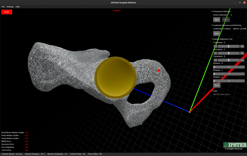
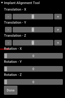
Figure 40. Landmark Registration in the Surgeon UI

Implant Alignment Tool

Prior to surgery, surgeons use the patient’s pelvic scan to plan the placement of the implant cup. Normally, the planning process is done on medical software that allows loading and viewing 3D models of the pelvis scan and implant.

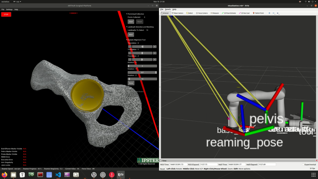
To replicate this, we developed a UI based on Open3D. This UI is able to load the pelvis scan and implant. Using the GUI library, we developed a frontend that allows the surgeon to perform several 3D transformations to the cup implant in order to plan its placement.

FIgure 41. Implant Alignment Toolbox for Adjusting Cup Placement

Integration with Watchdog and Controls Subsystems

The UI is integrated with the Watchdog module via ROS. The Watchdog publishes important system health information like the visibility of markers, robot arm singularity, joint limit states, and so on. The UI is able to display this information in real time by subscribing to the respective watchdog topics. If the Watchdog detects any system malfunction, the UI displays the error through a popup shown in the figure below.

Figure 42A. UI Showing Errors Published by Watchdog

Figure 42C. The Popup of the Watchdog Error

Once the implant alignment is complete, the UI calculates a relative transformation between the pelvis scan and implant. This relative transformation is then transformed into the camera frame and published as the camera to reaming_pose transform using ROS. The controls subsystem is able to continuously look up this transformation and align itself to the initial reaming position and orientation.

Figure 43. Integration Between UI and Watchdog/Controls Subsystems, Publishing the Desired Reaming Pose From UI

Spring 2022 Design Archive (Deprecated)

Motion Planning Subsystem

The planning node is responsible for generating linear trajectories between the current pose of the robot and the reaming end point. Using the free motion mode, the surgeon is expected to bring the tool closer to the site of surgery, after which the controller aligns the orientation of the end-effector with the reaming end point. The planning node operates after this realignment and passes the trajectory generated to the controller.

Setting Up IKFast

The default kinematics solver in MoveIt! is KDL and this was changed to IKFast. IKFast was preferred over KDL as IKFast is an analytical solver and is computationally efficient in comparison to KDL which is a numerical solver. As latency is an important consideration in our system, faster and deterministic solvers were preferred. The number of successful and unique solutions found by IKFast is much higher than KDL.

A docker image based on Ubuntu 14.04 and ROS Indigo was loaded and the robot URDF was passed to generate the IKFast plugin.

Setting Up Pilz Industrial Motion Planner

For planning, we use the Pilz industrial motion planner within MoveIt!. The Pilz planner essentially works as a trajectory generator and provides analytical solutions for the requested trajectory. The planner is successful in providing repeatable and deterministic solutions. The planner is also complemented by IKFast, which is an analytical inverse kinematics solver. The plan generated for our ARTHuR system is with respect to the robot base.

The default motion planner in MoveIt! is the Open Motion Planning Library (OMPL). OMPL uses sampling based algorithms which leads to non-deterministic motions between the same set of points. As the task at hand was to generate trajectories alone without having to do collision checking, we moved to using Pilz Industrial Motion Planner.

Upon installing the Pilz planner, changes had to be made to move group set up and launch files to recognize Pilz as a planning pipeline and load it as the default planner. Files were created to set the cartesian limits within which the planner should operate.

Figure 14. Motion Planning Using the Pilz Industrial Motion Planner

Writing a Node for Trajectory Generation

The kortex driver written by Kinova automatically loads when an arm is connected to a computer. For the compA ROS node was written in python to generate arbitrary trajectories between the current state and a random valid end-point. These functions were set up within a class along with other functions to get the current state, publish the generated trajectory, move the robot to goal pose in simulation etc. A custom ROS message was created to send the trajectory information to the controls node which included joint states and end-effector cartesian states for each waypoint in the generated trajectory. This message was then published to the controller at 10Hz via a topic.

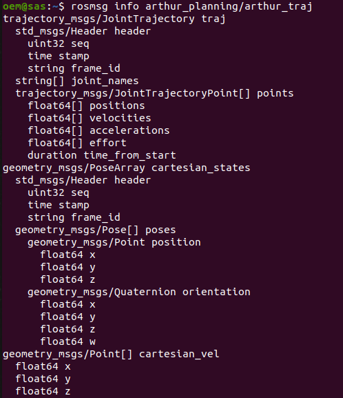
Writing a Custom ROS Message

To transfer the information of the generated trajectory, we created a custom ROS message type as seen in the figure below. The message consists of the joint trajectory message, pose array, point and an int32. The joint trajectory message holds information of the joint positions, velocities and accelerations at each waypoint in the trajectory. The pose array holds the cartesian states of the end-effector, namely the 3D position and orientation (in quaternion) of the tooltip. The list of point messages holds the cartesian velocities at each waypoint. Finally, we also have an integer variable called ‘trajNum’ which is used to keep track of the number of trajectories generated from the beginning and helps in dynamic compensation.

Figure 16. Custom ROS Message for all Necessary Trajectory Information

The joint state information could be directly accessed using MoveIt! function calls. The cartesian states had to be computed by calculating forward kinematics of the joint positions at each waypoint. The cartesian velocities were calculated using simple arithmetic i.e. dividing the difference of two consecutive cartesian positions by the time period. The Pilz planner is forced to plan a linear path in cartesian space while satisfying the joint limits specified by Kinova.

Whilst the system is in dynamic compensation mode, the controller realigns the end-effector to the new position of the pelvis. After this, a flag is sent to the planner to re-plan the trajectory from the robot’s current pose. At this point, the new current position is used to again plan a linear path to the new reaming endpoint in space.

Controls Subsystem

Connecting Kinova Gen3 with the Desktop

Controller

Free Motion Mode

Autonomous Control Mode

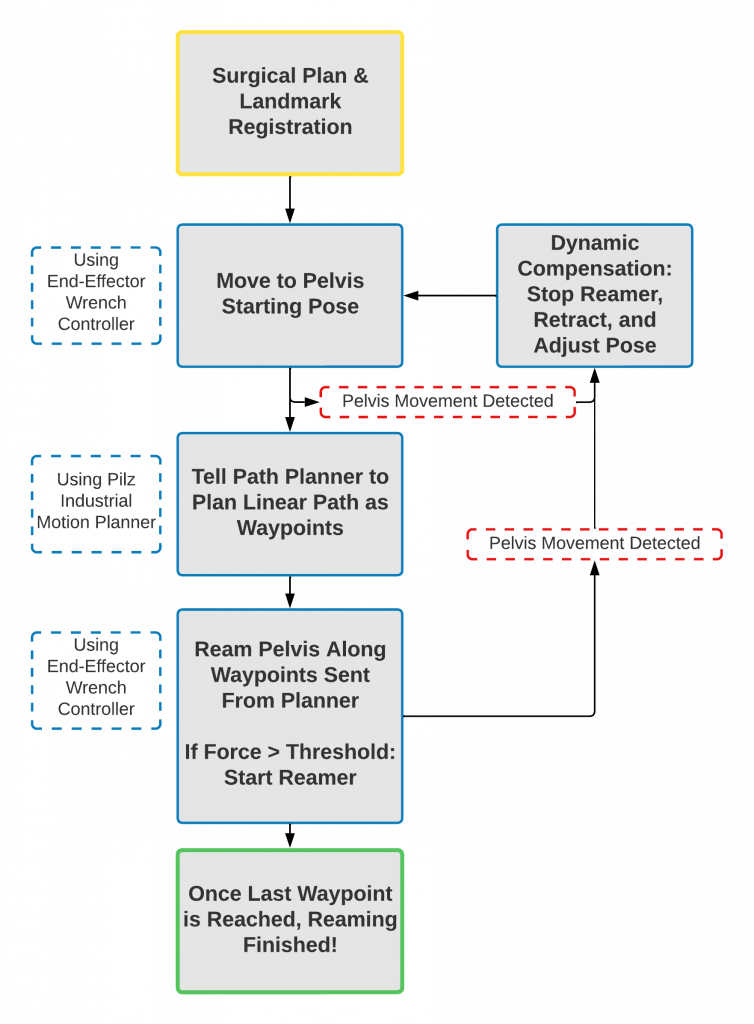
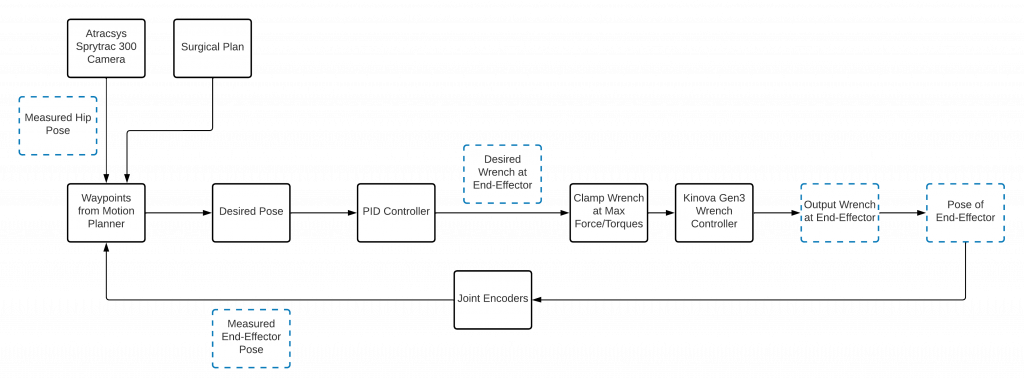
For Autonomous Control Mode, the controls subsystem is currently taking advantage of Kinova’s Wrench Command API built into their system. Essentially, our subsystem can send wrench commands to the arm, which moves the arm with respect to chosen frames. For our system, we are using a mixed frame, where the forces we send in the wrench command are with respect to the base frame coordinates, while the torques we send in the wrench command are with respect to the end-effector frame. The trajectory given by the motion planner has several waypoints containing desired positions and orientations for the end-effector to move through. Using this framework, a PID controller was developed which takes the error between the current pose and desired pose as the input into the PID controller, and outputs the desired wrench to reach that desired pose. The output of the PID controller is then clamped at a max force of 20 Newtons and max torque of 8 Nm. This allows the controller to be more safe around humans as the wrench controller will only exert these maximum forces in worst-case scenario. The figures below show the general flow diagram of how the Autonomous Control Mode moves through different states, and the control block diagram of the wrench controller, which takes the desired pose as the input (determined by the planner, camera, and surgical plan), and takes the actual pose of the end-effector as feedback.

Figure 18. Wrench Controller Block Diagram

Because the motion planner can only plan from the current position of the end-effector, the controller has to first align its orientation with the reaming endpoint frame (usually determined in the surgical plan pre-surgery) and moves to a point 5 cm axially from the reaming endpoint frame. once it is properly aligned at the reaming start point, the controller tells the planner to generate a trajectory and then proceeds to move along the trajectory using the PID controller described earlier.

Figure 19. Reamer Aligning to Reaming Starting Point

Once the reamer makes contact with the acetabulum and exerts a force above a tuned threshold (detected by the force/torque sensor), the controller communicates with the reaming node to start the reamer. The reason to start reaming only after making full contact with the acetabulum is that reaming before making full contact can introduce high amplitude vibrations into the system, reducing accuracy. Waiting for full contact will allow reaction forces from the bone to cancel out, reducing vibrations. Once the end-effector reached all waypoints, the reaming operation is finished and the arm retracts.

Figure 20. Reamer Starting Once Force Applied

Dynamic Compensation

For Dynamic Compensation, the perception system will notify the controls subsystem when the pelvis pose has changed beyond a specific threshold as specified by our requirements. When dynamic compensation is triggered, the arm retracts 10 cm along the axis of reaming, and then reorients itself to the reaming start point as described above. The controller is constantly keeping track of 10 cm behind its current end-effector pose, so that when dynamic compensation occurs, it knows where to retract to. After reorienting itself, it then gets a new trajectory and begins reaming again. Dynamic Compensation is demonstrated in the figure below.

Designing the Reaming End-Effector

The reaming end-effector design went through several evolutions throughout the project, as can be seen in the figure below. Originally we thought to clamp around the connection to the fiducial marker on the reamer handle, but we were advised by our sponsor to instead try to connect around the ridges of the reamer handle. We designed and 3D printed this design, but upon integration we determined that the design was too long which caused some undesirable wobbliness in the system. Based on this, we decided to stop trying to implement the reamer handle in our design, and instead create a 3D printed design which mimics the geometry of the reamer handle.

This led to our finalized design which can be seen in the figure below. This design featured three 3D printed parts, an adapter between the end-effector and the force-torque sensor, and a motor mount can hold a motor and mimic important geometries from the reamer handle, and a reamer head adapter. This final reaming end-effector worked perfectly for what we needed, as the assembly vibrated minimally during the procedure (most vibrations were through the entire arm) and the system was able to hold up to the torques during and operation. While we would like to pursue potential improvements to this system in the future, we are satisfied overall with this design.

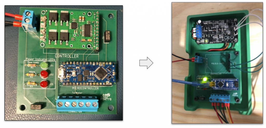
Designing the PCB

The PCB design went through a few iterations as well throughout the semester as can be seen in the figure below. Originally our system was designed to work with an Arduino nano and a Pololu 1457 on the same PCB board, allowing us to control the speed of the motor with PID velocity control utilizing the motors encoders. However, due to some short circuiting issues as a result of poor use of flux and malfunctioning components (Pololu 1457), we had to redesign the PCB to move the motor controller off the PCB. We decided to use the Cytron MD10C instead of the Pololu 1457, and using some jumper wires, were able to implement the Cytron into the system and utilize it as we planned to use the Pololu. With this completed, we developed some control code for the arduino, which we based on our prior work in the sensors and motors lab. The end result was that when the PCB was powered with an external power supply, our computer was able to control the reamer velocity via a rostopic and that velocity would be maintained regardless of the torque.

Assembling Final Hardware System

One final hardware task we would like to highlight is the set-up of the force-torque sensor. The force-torque sensor was powered using the same power supply as the reamer motor, and it was communicated with via a provided Ethernet cable. There were several methods of communicating with the force torque sensor, but the most consistent for us was logging into the sensor via a telnet session and requesting the forces and torques at a frequency of around 60 Hz. Implementing these values received from the telnet session into a ROS node allowed us to publish the resulting values to rostopics. One issue with this set-up is how the values are biased, as the values are initially biased at start-up to eliminate the forces and torques as a result of the connection to the end-effector. However, these values change, leading forces and torques being recorded when there are none acting on the system. This led to a bug in our system which caused the reamer motor to turn on early when it should have only turned on when the end-effector contacted the pelvis. To prevent this bug we would like to improve how we are handling the biasing of the data in the future. A picture of the finalized hardware system can be seen in figure 27.