The perception subsystem consists of Localization, State Estimation and Obstacle detection and tracking.

Localization 

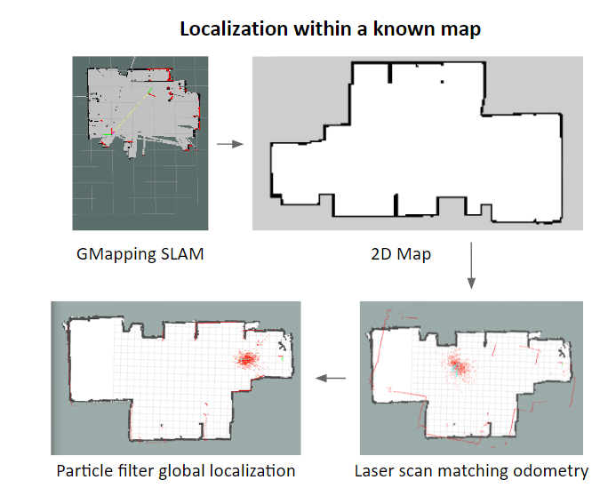
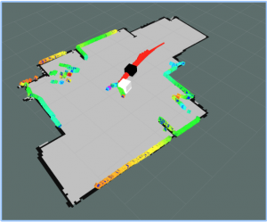
Our final localization implementation allows to keep track of the robot’s pose and states reliably under fast motions and rotations, as shown below.

 

The localization subsystem consists of our sensors and localization algorithms. Currently we have two sensors on the robot: an inertial measurement unit and a Hokuyo UST-10LX laser scanner. The LIDAR provides most of the information for our localization algorithms, with a 270o field-of-view on a single plane at 40 Hz.

While we were able to get wheel odometry information from the VESC, this information becomes unreliable once the wheel speeds go above 2m/s, where there is significant wheel slip. Hence, we required an alternate means of odometry, and we found that a laser scan matching framework using data from the LIDAR provided decent results. Using the laser_scan_matcher ROS package, we spent some time tweaking the parameters to fit our purposes, and was able to obtain reliable odometry at up to 30 Hz, regardless of wheel slip.

Despite having a decent source of odometry, laser scan matching is not perfect, and will start to accumulate drift when the robot is moving or rotating at high speeds. We needed a way to localize globally within our known map, and we opted for a particle filter localization technique.

We used the third-party ROS package amcl, which stands for Adaptive Monte Carlo Localization for this purpose. Given the known map provided from the map_server, AMCL then uses this known map to localize itself. Since we are not doing SLAM, there is no uncertainty associated with the map, and AMCL is able to give us more robust localization in our known environment then performing SLAM in real-time.

For the purpose of building the map, we leveraged the open-source ROS package gmapping, using the laser scan matcher as our odometry source. We also post-processed the map in an image editing software to remove outliers and spurious points to ensure robust localization.

 

 

Making a map of our lab space

AMCL in our lab space

 

 

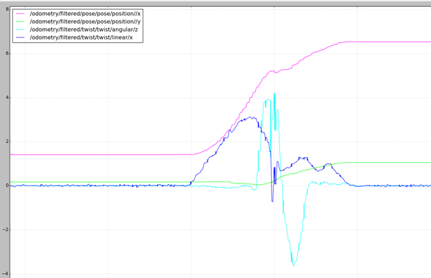
In addition to knowing the pose of the robot, we also needed an accurate estimate of the linear and angular velocities of the robot. We used the robot_localization ROS package for this, which implements an Extended Kalman Filter to estimate the linear (longitudinal and lateral) and angular velocities of the robot. This information is crucial for our planner to be able generate a feasible trajectory when  avoiding an obstacle. Additionally, we were also able to use it to verify that our robot is reaching the desired initial velocity of 3m/s before reacting to the obstacle.

Plot of EKF state estimate

 

 

Obstacle Detection And Tracking

The Obstacle Detection And Tracking stack consists of three major components: clustering, data association and state estimation (using a Kalman Filter). 

Clustering uses a KD-Tree to parse through the point cloud and cluster the data, within a specified tolerance radius. Data association uses the Euclidean Distance algorithm to  estimate the cluster center position and velocity for tracking the clusters.

Methodology

We initialize the tracking algorithm with Kalman Filter Objects (part of OpenCV Library). After noise removal, the point cloud is clustered into Regions of Interest. The Regions of Interest are determined on the basis of the size of the clusters. If the size of the cluster is too huge (on the order of 500 – 600 point), it is definitely not an obstacle representing a vehicle or a human (given our setup). Subsequently, each of the Regions of Interest (clusters) is assigned an Object Identifier number . The object Identifier number stores the cluster center for the cluster recognition. The tracker uses the Centroid of the Cluster for re-assigning the Object Identification Number from one frame to the next.

The tracking problem comprises of two main steps:

Data Association

The data association is done by using the minimum Euclidean Distance Algorithm.  Let Object Identifier y be associated with cluster with centre x, at a given frame. In the next frame, the cluster whose center is closest (by Euclidean Distance) to x would be associated with the object Identifier y. This process is repeated for all the object identifiers, to get the cluster association from one frame to the next.

State Estimation and Prediction using Kalman-Filter algorithm

The 2-D point cloud is tracked with the help of its cluster centres. The Kalman Filter algorithm tracks the cluster center to track the clusters in the point cloud. The state dimension for the tracking is 4 i.e (position in x , position in y , velocity in x, velocity in y). The measurement matrix consists of 2 dimensions – velocity in x and velocity in y. There is no control input for the Kalman Filter (given our setup). At each time frame, it predicts the estimated position and velocities of the cluster centers and compares it to the observed state matrix to find out the Kalman Gain. The Kalman Gain is then used to update the covariance matrix and output the position and velocities of the cluster center.

The black cube represents Robot and the White cube represents obstacle.

    Obstacle Detection

In our final implementation, we had two variants of our obstacle detection and tracking module: the first was a full implementation that detects, clusters and tracks each obstacle, and the second was a time-optimal version that detects and fixes the obstacle position just once. While the full implementation worked really well, we opted for the time-optimal one for most of our tests as we wanted to minimize the delay between detection, planning and execution as much as we could.