Spring semester – Dynamic planning w/ trajectory optimization
To plan evasive maneuvers through tire slip, we used a trajectory optimization algorithm called control-limited iterative linear quadratic regulator (iLQR). iLQR is a dynamic-programming based shooting method that alternates between performing forward rollouts of a control policy, and passing backwards over the trajectory while calculating new control policies. We chose this algorithm for its conceptual simplicity, ability to encode complex constraints, and the fact that its intermediate trajectories are always dynamically feasible (meaning we could use this algorithm in an anytime/fixed-rate fashion, if needed).
As with most other trajectory optimization algorithms, we defined the desired behavior of the robot in the cost function. We imposed costs for distance to the goal state, proximity to the obstacle, and control inputs.
The goal state cost was formulated as a weighted linear combination of the difference between the robot’s current state and its goal state. This cost encourages the robot to get close to the goal state as quickly as possible.
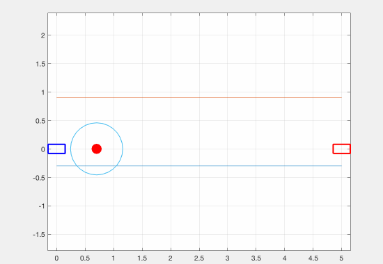
The obstacle cost was formulated as a dynamic potential field. The dynamic potential field accounts for not only the position of the robot relative to the obstacle, but its velocity as well. The robot is penalized for the magnitude and direction of its velocity vector. For example, a velocity pointed straight towards the robot will be penalized much higher than a velocity pointed perpendicular to the robot-obstacle vector.
We also imposed a cost on change in controls. This encouraged the optimizer to find trajectories with smooth changes in controls, instead of jerky outputs that our robot may not be able to execute in reality.
Wherever there was an absolute value function in our cost function, we replaced it with a differentiable approximation to the absolute value function. This allowed iLQR to find a linear approximation of the cost function at each point in the state space.
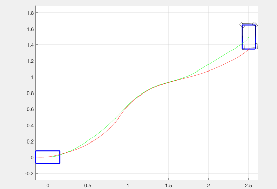
As an experiment, we also tried adding a negative cost (reward) for transverse velocity. This was meant to encourage the optimizer to find trajectories in which the robot was drifting. Although we weighted this down to be negligible in our final implementation, we believe that it was important to have this as an option. The effect of this term on the resulting trajectories is shown in the figure below.
During our initial simulation tests, we found that iLQR was fairly sensitive to initial guesses for the control sequence. This is due to the divergent nature of the forward simulation used in the algorithm. To ensure that our solution trajectory was reasonable, we initialized our optimization with a control sequence recorded from a manual (controlled by human with joysticks) maneuver.
We implemented the vehicle controller in ROS. We separated the controller into two components: a trajectory generator/planner, and a trajectory executer. The trajectory generator is responsible for switching between our planners (ramp-up and iLQR), reacting to external events (obstacles, user commands), and sending trajectories to the executor. The executor sends control commands to the servo and ESC at a specified rate, and provides closed loop trajectory tracking. Using ROS actionlib, the trajectory generator (action client) is able to preempt a trajectory that is currently being executed by the executor (action server). This architecture gave us the ability to switch between plans seamlessly.
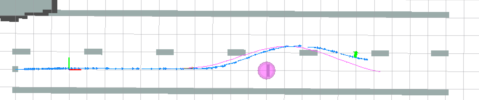
In our final implementation, we were able to generate a plan on-board with the iLQR planner within 0.08s, while performing low-level closed loop control at 20 Hz. In most cases, the robot is able to track the prescribed trajectory fairly well. As shown below, we generate a plan (shown in purple) once the obstacle is detected, and the robot follows the plan to avoid the obstacle (robot odometry shown in blue), with minimal delay between planning and execution.
Fall semester – Kinematic planning
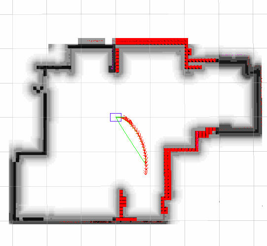
For path planning we use the ROS Navigation stack as our framework. The Navigation stack takes in sensor, odometry, map data as inputs, and provides planning as an output. A node graph is shown below:
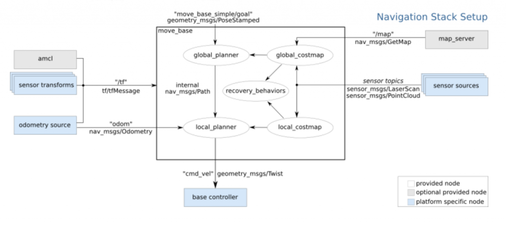
The Navigation stack provides the ability to swap our global and local planners as plugins, using a common interface. We are using the stock global planner, which uses Djikstra’s algorithm to search over the global costmap. For local planning, we are using the Timed Elastic Band algorithm developed at TU Dortmund.
The local planner sends velocity commands to our custom base controller node, which converts the velocity command into an Ackermann steering and throttle format. This message is passed to the Teensy, which provides low-level control of the robot’s drive system.
Below, you can see our global and local planners working in sim. The green line represents the global planner; it simply looks for the shortest path from the base link to the goal, and does not consider any of the kinematic constraints of our robots. This is taken care of by our local planner, which solves an optimization problem to find the minimum-time path to the goal point, given our global plan and kinematic constraints.