Leader Detection and Pose Estimation
This subsystem serves to extract information about the leader Zamboni ice resurfacer that can be used together with the follower’s information to generate a trajectory to follow. To facilitate robust detection and pose estimation in our particular setup, we take advantage of ArUco markers instead of using a object detection network (e.g. YOLO3D). The subsystem is mainly composed of three major components: (1) individual marker detection, (2) marker board pose estimation, and (3) transform broadcasting.
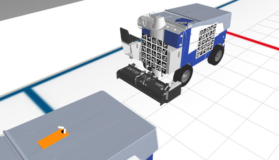
We attach three different marker boards, each one with a different ArUco dictionary so that the camera can distinguish among them, on the leader, one on the left, one at the rear, and one on the right. Also, to get a wider field of view (FoV) so that we will not lose track of the markers when the leader is taking a turn, we set up two cameras in a shape of “Λ”. Figure 1 above illustrates such a setting.
We leverage the ArUco library from OpenCV to detect individual markers as well as estimating the pose of the marker boards. In particular, individual markers are first detected on the image returned by each camera, given the specific ArUco dictionary associating with each board. The pose estimation is performed using the detected markers on boards that can be observed in the camera image. Therefore, there will be at most 6 possible combinations of pose estimations (2 camera images X 3 boards) during every callback. We determine the best one to be used for the final pose based on the number of markers detected. That is, for each pair of camera images, we use the one that detects the most number of markers; and for all of the three possible boards, we use the one that returns the most number of markers across all pairs of camera images. Finally, since the pose returned is the transform from the board frame to the camera frame, we chain the transform with the one from the board (that is used for final pose estimation) to the leader base, and broadcast the transform (from the camera that is used for final pose estimation to the leader base) after converting it from OpenCV conventions to ROS tf conventions.
An example video of the initial prototype with only one camera and one marker board is shown below. The pose estimate is drawn as an axis on the left bottom corner in the RGB image. In the terminal, the Interpolated Average Depth is the average depth values in the Depth image after masking it with all the markers detected in the RGB image, while the Translation Norm is the norm of the translation vector returned in the pose estimate.
Another video below shows the leader pose estimation using the two-camera setup with three marker boards on the leader. The top right terminal is calculating the rotation and translation difference between the estimated leader base and the ground truth leader base. The errors are very small for both translation and rotation.
Filtering
When the system is tested in real world, we find that the leader pose estimated is unstable and wobbling, especially when the leader becomes farther or the follower vibrates due to roughness of the ground. Therefore, we implement a Kalman-like temporal filtering to filter out outliers in pose estimations. This makes the perception subsystem robust against both occlusions and motion blur. Occlusions happen a lot when the leader is turning. Motion blur is mainly caused by the low frame rate under limited bandwidth of the computing unit. The robustness also leaves more leniency for downstreaming modules, especially planning and control.
Our approach can be summarized as follows:
- Estimate Step (without any ArUco marker detected)
- Extrapolate linear positions by fitting curves on a fixed window of previous poses with sampling or sparsifying
- Extrapolate rotations by RotationSpline from SciPy
- Update Step (with ArUco marker detection)
- Option 1 – fuse the current state with estimated pose from ArUco
- Problem: accumulation of errors
- Option 2 – directly use the estimated pose from ArUco
- Problem: relying on the accuracy of the extrapolation
- Option 1 – fuse the current state with estimated pose from ArUco
In the estimate step, the main idea is extrapolation based on the history of poses. Since we use a fixed window, say, with a window size of K, we shall not use any previous K poses from the current timestamp. This works fine when the leader is moving straight ahead but it fails when the leader starts turning, because the previous K poses are very close to each other due to the high frame rate of the camera and hence they tend to accumulate in the same place. Extrapolation on these poses won’t give reasonable predictions. Instead, we should extrapolate based on poses in the past K seconds, and this is where sampling/sparsifying comes into play.
In the update step, we can implement a Kalman filter, which means we filter the prediction with the measurement, i.e. true positive ArUco marker detections. However, this comes with the problem of error accumulation because we need to assign the prediction with the belief as how we trust the prediction. On the other hand, we can directly use the measurement. The downside is that if the extrapolation is not accurate enough, there will discontinuity between predicted poses and updated poses. We end up with the second option because we have successful implementation of path smoothing and curve fitting in the planning subsystem, which means small discontinuity in perception will not break the system. We show the filtering results below.
Obstacle Detection
We implement obstacle detection so that the Zamboni vehicle will stop automatically whenever there’s an obstacle blocking its way, i.e. inside its 30-degree FoV.
We use an off-the-shelf MobileNet SSD (Single Shot Multibox Detector), which is lightwetight and optimized on edge devices so that we do not need an extra GPU to run this subsystem. We restrict the output categories of the network to be the objects that will appear in an ice rink only, e.g. person, gate. Anytime when there’s an object belonging to any of these categories being detected, the braking command will be sent to ECU and the Zamboni will stop itself. Result is shown below.
Leader Detection with LiDAR (Archived)
In addition to this, we have also made a prototype that uses a 360-degree LiDAR instead of a two-camera setup to enhance the FoV. The pipeline is as follows:
1. Conversion: The ROS PointCloud2 message (published by the Velodyne’s Puck in Gazebo) is first converted to a Point Cloud Library (PCL) XYZRGB format, with the “ring” field converted to a corresponding RGB value.
2. Filtering: The point cloud is downsampled using voxel grid filter in PCL. Then it will be filtered based on three different axes using the passthrough filter in PCL. In our case, I filter it along 𝑧 from −ℎ to 0 where ℎ is the height of the Puck from the ground, along 𝑥 from −5 to 10 which approximates the farthest longitudinal distance between the leader and the sensor, and along 𝑦 from −5 to 5 which approximates the farthest lateral distance.
3. Plane Segmentation (Optional): if the filtering along 𝑧 still gives a lot of points on the ground, then the point cloud is segmented using a RANSAC plane segmenter in PCL. The inliers will be the plane while the outliers will be the follower, the leader, and any random obstacles.
4. Clustering: The PCL XYZRGB point cloud is converted to a XYZ point cloud first because Euclidean clustering does not need RGB information. Then an Euclidean clustering is applied to the points, which in the backend uses a Kd-tree to find the nearest neighbors (further details are well explained here). After getting a list of clusters, I assign a color to each cluster of points.
5. Conversion: The downsampled, filtered, and clustered point cloud is converted back to a ROS PointCloud2 message which includes the corresponding cluster color as a PointField. The RViz can now show the clustered data with colors.
6. Pose Estimation: A robust pose estimation of rigid objects will be performed on the leader’s point clouds by matching them with a ground truth leader point clouds.
The video above shows the point clouds after filtering processing. On the right we can see only the points around the leader and the follower are remaining. This approach of using LiDAR is still being investigated and needs further testing and validation. For the moment, we are using the two-camera setup for the following subsystems, i.e., waypoint generation and localization.
LiDAR-Camera Fusion (Archived)
We also tried LiDAR-camera fusion for obstacle detection. We stopped the implementation after calibration due to time constraints and we narrowed our scope to camera-based detection, as shown above, which is robust enough and satifies the system requirements. Our goal is to detect any object in the image space using popular detectors such as YOLO, project the point cloud from the LiDAR onto the image, and extract the 3D positions of the object. Note that this approach is straightforward if we need to avoid the obstacle, but the specification from one of the stakeholders, Penguins, requires us to merely stop the vehicle until the object is removed from the path. Therefore, camera-bsed detection suffices in our case. We still document our approach to LiDAR-camera fusion here.
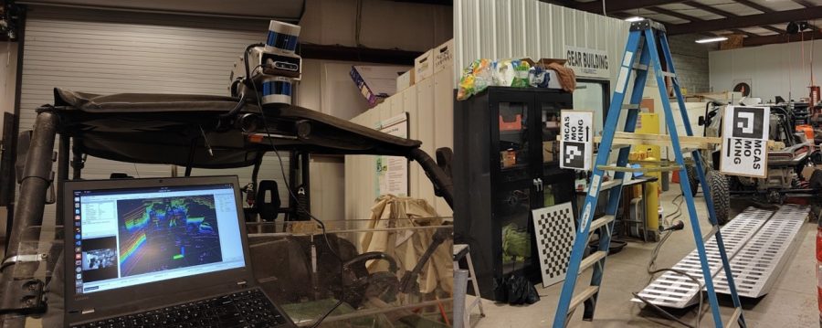
To fuse the two modalities, we need to calibrate them first. We use the popular ROS package to automatically calculate the initial extrinsics and then manually finetune it using a GUI-based calibration tool. The figure below shows the setup for the auto calibration.
To start iterative LiDAR-camera calibration using 3D-3D point correspondences, we mark each edge of the board. Each board have 4 line segments and need to be marked from leftmost board to the rightmost board. We draw a quadri-lateral around the line of points that we believe correspond to an edge of a board in the grayscale image. After annotating all the line segments, the rigid body transformation between the camera and the LiDAR frames will be calculated with a fixed number of iterations (50 by default). It also calculates the Root Mean Squared Error (RMSE) between the 3D points viewed from the camera and the laser scanner after applying the calculated transformation.